6.6: Standing Waves/VSWR

Last updated
Save as PDF

Page ID: 88578

$ \newcommand{\vecs}[1]{\overset { \scriptstyle \rightharpoonup} {\mathbf{#1}} } $

$ \newcommand{\vecd}[1]{\overset{-\!-\!\rightharpoonup}{\vphantom{a}\smash {#1}}} $

$ \newcommand{\id}{\mathrm{id}}$ $ \newcommand{\Span}{\mathrm{span}}$

( \newcommand{\kernel}{\mathrm{null}\,}\) $ \newcommand{\range}{\mathrm{range}\,}$

$ \newcommand{\RealPart}{\mathrm{Re}}$ $ \newcommand{\ImaginaryPart}{\mathrm{Im}}$

$ \newcommand{\Argument}{\mathrm{Arg}}$ $ \newcommand{\norm}[1]{\| #1 \|}$

$ \newcommand{\inner}[2]{\langle #1, #2 \rangle}$

$ \newcommand{\Span}{\mathrm{span}}$

$ \newcommand{\id}{\mathrm{id}}$

$ \newcommand{\Span}{\mathrm{span}}$

$ \newcommand{\kernel}{\mathrm{null}\,}$

$ \newcommand{\range}{\mathrm{range}\,}$

$ \newcommand{\RealPart}{\mathrm{Re}}$

$ \newcommand{\ImaginaryPart}{\mathrm{Im}}$

$ \newcommand{\Argument}{\mathrm{Arg}}$

$ \newcommand{\norm}[1]{\| #1 \|}$

$ \newcommand{\inner}[2]{\langle #1, #2 \rangle}$

$ \newcommand{\Span}{\mathrm{span}}$ $ \newcommand{\AA}{\unicode[.8,0]{x212B}}$

$ \newcommand{\vectorA}[1]{\vec{#1}} % arrow$

$ \newcommand{\vectorAt}[1]{\vec{\text{#1}}} % arrow$

$ \newcommand{\vectorB}[1]{\overset { \scriptstyle \rightharpoonup} {\mathbf{#1}} } $

$ \newcommand{\vectorC}[1]{\textbf{#1}} $

$ \newcommand{\vectorD}[1]{\overrightarrow{#1}} $

$ \newcommand{\vectorDt}[1]{\overrightarrow{\text{#1}}} $

$ \newcommand{\vectE}[1]{\overset{-\!-\!\rightharpoonup}{\vphantom{a}\smash{\mathbf {#1}}}} $

$ \newcommand{\vecs}[1]{\overset { \scriptstyle \rightharpoonup} {\mathbf{#1}} } $

$ \newcommand{\vecd}[1]{\overset{-\!-\!\rightharpoonup}{\vphantom{a}\smash {#1}}} $

$\newcommand{\avec}{\mathbf a}$ $\newcommand{\bvec}{\mathbf b}$ $\newcommand{\cvec}{\mathbf c}$ $\newcommand{\dvec}{\mathbf d}$ $\newcommand{\dtil}{\widetilde{\mathbf d}}$ $\newcommand{\evec}{\mathbf e}$ $\newcommand{\fvec}{\mathbf f}$ $\newcommand{\nvec}{\mathbf n}$ $\newcommand{\pvec}{\mathbf p}$ $\newcommand{\qvec}{\mathbf q}$ $\newcommand{\svec}{\mathbf s}$ $\newcommand{\tvec}{\mathbf t}$ $\newcommand{\uvec}{\mathbf u}$ $\newcommand{\vvec}{\mathbf v}$ $\newcommand{\wvec}{\mathbf w}$ $\newcommand{\xvec}{\mathbf x}$ $\newcommand{\yvec}{\mathbf y}$ $\newcommand{\zvec}{\mathbf z}$ $\newcommand{\rvec}{\mathbf r}$ $\newcommand{\mvec}{\mathbf m}$ $\newcommand{\zerovec}{\mathbf 0}$ $\newcommand{\onevec}{\mathbf 1}$ $\newcommand{\real}{\mathbb R}$ $\newcommand{\twovec}[2]{\left[\begin{array}{r}#1 \\ #2 \end{array}\right]}$ $\newcommand{\ctwovec}[2]{\left[\begin{array}{c}#1 \\ #2 \end{array}\right]}$ $\newcommand{\threevec}[3]{\left[\begin{array}{r}#1 \\ #2 \\ #3 \end{array}\right]}$ $\newcommand{\cthreevec}[3]{\left[\begin{array}{c}#1 \\ #2 \\ #3 \end{array}\right]}$ $\newcommand{\fourvec}[4]{\left[\begin{array}{r}#1 \\ #2 \\ #3 \\ #4 \end{array}\right]}$ $\newcommand{\cfourvec}[4]{\left[\begin{array}{c}#1 \\ #2 \\ #3 \\ #4 \end{array}\right]}$ $\newcommand{\fivevec}[5]{\left[\begin{array}{r}#1 \\ #2 \\ #3 \\ #4 \\ #5 \\ \end{array}\right]}$ $\newcommand{\cfivevec}[5]{\left[\begin{array}{c}#1 \\ #2 \\ #3 \\ #4 \\ #5 \\ \end{array}\right]}$ $\newcommand{\mattwo}[4]{\left[\begin{array}{rr}#1 \amp #2 \\ #3 \amp #4 \\ \end{array}\right]}$ $\newcommand{\laspan}[1]{\text{Span}\{#1\}}$ $\newcommand{\bcal}{\cal B}$ $\newcommand{\ccal}{\cal C}$ $\newcommand{\scal}{\cal S}$ $\newcommand{\wcal}{\cal W}$ $\newcommand{\ecal}{\cal E}$ $\newcommand{\coords}[2]{\left\{#1\right\}_{#2}}$ $\newcommand{\gray}[1]{\color{gray}{#1}}$ $\newcommand{\lgray}[1]{\color{lightgray}{#1}}$ $\newcommand{\rank}{\operatorname{rank}}$ $\newcommand{\row}{\text{Row}}$ $\newcommand{\col}{\text{Col}}$ $\renewcommand{\row}{\text{Row}}$ $\newcommand{\nul}{\text{Nul}}$ $\newcommand{\var}{\text{Var}}$ $\newcommand{\corr}{\text{corr}}$ $\newcommand{\len}[1]{\left|#1\right|}$ $\newcommand{\bbar}{\overline{\bvec}}$ $\newcommand{\bhat}{\widehat{\bvec}}$ $\newcommand{\bperp}{\bvec^\perp}$ $\newcommand{\xhat}{\widehat{\xvec}}$ $\newcommand{\vhat}{\widehat{\vvec}}$ $\newcommand{\uhat}{\widehat{\uvec}}$ $\newcommand{\what}{\widehat{\wvec}}$ $\newcommand{\Sighat}{\widehat{\Sigma}}$ $\newcommand{\lt}{<}$ $\newcommand{\gt}{>}$ $\newcommand{\amp}{&}$ $\definecolor{fillinmathshade}{gray}{0.9}$

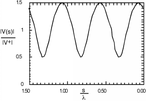
Standing wave pattern of the magnitude of V(s) divided by the magnitude of V+, plotted over a horizontal axis of the quotient of s and lambda. Wave crests reach 1.5 and troughs reach 0.5. The waves have a period of 0.5. — Figure $\PageIndex{1}$: A standing wave pattern

In making this plot, we have made use of the fact that the propagation constant $β$ can also be expressed as $\frac{2}{π}$ , and so for the independent variable, instead of showing $s$ in meters or whatever, we normalize the distance away from the load to the wavelength of the excitation signal, and hence show distance in wavelengths. What we are showing here is called a standing wave. There are places along the line where the magnitude of the voltage $| V (s) |$ has a maximum value. This is where $V^{+}$ and $V^{-}$ are adding up in phase with one another, and places where there is a voltage minimum, where $V^{+}$ and $V^{-}$ add up out of phase. Since $| V^{-} | = | Γ_{ν} | | V^{+} |$ , the maximum value of the standing wave pattern is $1 + | Γ_{ν} |$ times $| V^{+} |$ and the minimum is $1 - | Γ_{ν} |$ times $| V^{+} |$ . Note that anywhere on the line, the voltage is still oscillating at $e^{i ω t}$ , and so it is not a constant, it is just that the magnitude of the oscillating signal changes as we move down the line. If we were to put an oscilloscope across the line, we would see an AC signal, oscillating at a frequency $ω$ .

A number of considerable interest is the ratio of the maximum voltage amplitude to the minimum voltage amplitude, called the voltage standing wave ratio, or VSWR for short. It is easy to see that:

VSWR = \frac{1 + | Γ |}{1 - | Γ |}

Note that because $| Γ_{ν} | \in [0, 1]$ , $VSWR \in [1, \infty]$ .

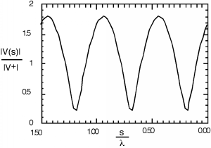
Although Figure $\PageIndex{1}$ looks like the standing wave pattern is more or less sinusoidal, if we increase $| Γ |$ to 0.8, we see that it most definitely is not. There is also a temptation to say that the spacing between minima (or maxima) of the standing wave pattern is $λ$ , the wavelength of the signal, but a closer inspection of either Figure $\PageIndex{1}$ or Figure $\PageIndex{2}$ shows that in fact the spacing between features is only half a wavelength, or $\frac{λ}{2}$ . Why is this? Well, $φ (s)$ goes as $-2 β s$ and $β = \frac{2 π}{λ}$ , and so every time $s$ increases by $\frac{λ}{2}$ , $φ (s)$ decreases by $2 π$ and we have come one full cycle on the way $| V (s) |$ behaves.

Graph of the standing wave pattern from Figure 1 above is repeated with the same period but a maximum height of 1.8 and minimum height of 0.2. The wave troughs are visibly narrower than the crests. — Figure $\PageIndex{2}$: Standing wave pattern with a larger reflection coefficient

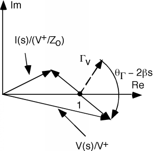
Now let's go back to the crank diagram. At the position shown, we are at a voltage maximum, and $\frac{Z (s)}{Z_{0}}$ just equals the VSWR.

\begin{array}{rcl} \frac{Z (s_{V_{\max}})}{Z_{0}} & = & VSWR \\ = & \frac{1 + | Γ_{ν} |}{1 - | Γ_{ν} |} \end{array}

Note also that at this particular point, that the voltage and current phasors are in phase with one another (lined up in the same direction) and hence the impedance must be real or resistive.

We can move further down the line, and now the $V (s)$ phasor starts shrinking and the $I (s)$ phasor starts to get bigger, as shown in Figure $\PageIndex{3}$.

Crank diagram which has rotated a short distance past V_max. — Figure $\PageIndex{3}$: Moving further down the line from a $V_{\max}$

If we move even further down the line, we get to a point where the current phasor is now at a maximum value, and the voltage phasor is at a minimum value, as seen in Figure $\PageIndex{4}$. We are now at a voltage minimum, the impedance is again real (the voltage and current phasors are lined up with one another, so they must be in phase) and

\begin{array}{rcl} Z (s_{V_{\min}}) & = & \frac{1}{VSWR} \\ = & \frac{1 - | Γ_{ν} |}{1 + | Γ_{ν} |} \end{array}

Crank diagram that has rotated 180 degrees from V_max, so that the vectors for V(s)/V+ and I(s)/(V+/Z_0) both lie on the real axis pointing away from the origin and the Gamma_v vector lies on the real axis pointing towards the origin. — Figure $\PageIndex{4}$: Moving even further down the line, with crank diagram at a $V_{\min}$

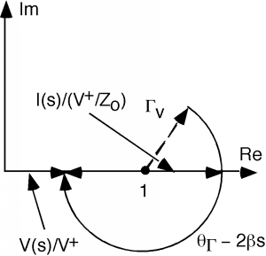
The only problem we have here is that except at a voltage minimum or maximum, finding $Z (s)$ from the crank diagram is not very straightforward, since the voltage and current are out of phase, and dividing the two vectors becomes somewhat tedious.

Search

Text Color

Text Size

Margin Size

Font Type