6.7: Bilinear Transform

There is a way that we can make things a good bit easier for ourselves, however. The only drawback is that we have to do some complex analysis first, and look at a bilinear transform! Let's do one more substitution, and define another complex vector, which we can call $r\left(s\right)$:

$$r\left(s\right)\equiv \left|{\Gamma }_{\nu }\right|e^{i({\theta }_r-2\beta s)}$$

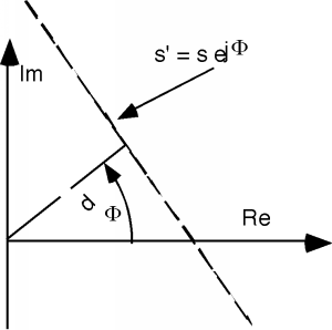
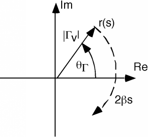
The vector $r\left(s\right)$ is just the rotating part of the crank diagram which we have been looking at, which is labeled in Figure \(\PageIndex{1}\). It has a magnitude equal to that of the reflection coefficient, and it rotates around at a rate $2\beta s$ as we move down the line. For every $r\left(s\right)$ there is a corresponding $Z\left(s\right)$ which is given by:

$$Z\left(s\right)=Z_0\frac{1+r\left(s\right)}{1-r\left(s\right)}$$

Figure \(\PageIndex{1}\): The vector r(s)

Now, it turns out to be easier if we talk about a normalized impedance, which we get by dividing $Z\left(s\right)$ by $Z_0$.

$$\frac{Z\left(s\right)}{Z_0}=\frac{1+r\left(s\right)}{1-r\left(s\right)}$$

which we can solve for $r\left(s\right)$

$$r\left(s\right)=\frac{\frac{Z\left(s\right)}{Z_0}-1}{\frac{Z\left(s\right)}{Z_0}+1}$$

This relationship is called a bilinear transform. For every $r\left(s\right)$ that we can imagine, there is one and only one $\frac{Z\left(s\right)}{Z_0}$ and for every $\frac{Z\left(s\right)}{Z_0}$ there is one and only one $r\left(s\right)$. What we would like to be able to do, is find $\frac{Z\left(s\right)}{Z_0}$, given an $r\left(s\right)$. The reason for this should be readily apparent. Whereas, as we move along in $s$, $\frac{Z\left(s\right)}{Z_0}$ behaves in a most difficult manner (dividing one phasor by another), $r\left(s\right)$ simply rotates around on the complex plane. Given one $r\left(s_0\right)$ it is easy to find another $r\left(s\right)$. We just rotate around!

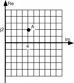
We shall find the required relationship in a graphical manner. Suppose I have a complex plane, representing $\frac{Z\left(s\right)}{Z_0}$. And then suppose I have some point \(A\) on that plane and I want to know what impedance it represents. I just read along the two axes, and find that, for the example in Figure \(\PageIndex{2}\), \(A\) represents an impedance of $\frac{Z\left(s\right)}{Z_0}=4+2i$. What I would like to do would be to get a grid similar to that on the $\frac{Z\left(s\right)}{Z_0}$plane, but on the $r\left(s\right)$ plane instead. That way, if I knew one impedence (say $\frac{Z\left(0\right)}{Z_0}=\frac{Z_L}{Z_0}$) then I could find any other impedance, at any other $s$, by simply rotating $r\left(s\right)$around by $2\beta s$, and then reading off the new $\frac{Z\left(s\right)}{Z_0}$ from the grid I had developed. This is what we shall attempt to do.

Figure \(\PageIndex{2}\): The complex impedance plane

Let's start with Equation and re-write it as:

$$\begin{array}{rcl}\hfill r\left(s\right)& \hfill =\hfill & \frac{\frac{Z\left(s\right)}{Z_0}+1-2}{\frac{Z\left(s\right)}{Z_0}+1}\hfill \\ \hfill & \hfill =\hfill & 1+\frac{-2}{\frac{Z\left(s\right)}{Z_0}+1}\hfill \end{array}$$

In order to use Equation, we are going to have to interpret it in a way which might seem a little odd to you. The way we will read the equation is to say: "Take $\frac{Z\left(s\right)}{Z_0}$ and add 1 to it. Invert what you get, and multiply by -2. Then add 1 to the result." Simple, isn't it? The only hard part we have in doing this is inverting $\frac{Z\left(s\right)}{Z_0}+1$. This, it turns out, is pretty easy once we learn one very important fact.

The one fact about algebra on the complex plane that we need is as follows. Consider a vertical line, $s$, on the complex plane, located a distance $d$ away from the imaginary axis as in Figure \(\PageIndex{3}\). There are a lot of ways we could express the line $s$, but we will choose one which will turn out to be convenient for us. Let's let:

$$s=d(1-i$$tanφ) ∀ φ :φ∈ −π2 π2 s d 1 φ φ φ 2 2

Figure \(\PageIndex{3}\): A vertical line, s, a distance, d, away from the imaginary axis

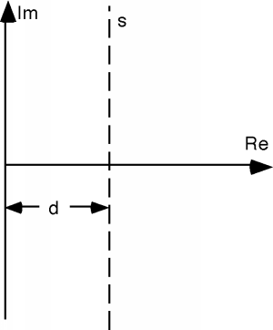
Now we ask ourselves the question: what is the inverse of s?

$$\frac{1}{s}=\frac{1}{d}\frac{1}{1-i}$$tanφ 1 s 1 d 1 1 φ

We can substitute for $$tanφ φ :

$$\begin{array}{rcl}\hfill \frac{1}{s}& \hfill =\hfill & \frac{1}{d}\frac{1}{1-i\frac{}{}}\hfill \end{array}$$sinφcosφ=1d⁢cosφcosφ−i⁢sinφ 1 s 1 d 1 1 φ φ 1 d φ φ φ

And then, since $$cosφ−i⁢sinφ=e−(i⁢φ) φ φ φ

$$\begin{array}{rcl}\hfill \frac{1}{s}& \hfill =\hfill & \frac{1}{d}\frac{}{}\hfill \end{array}$$cosφe−(i⁢φ)=1d⁢cosφ⁢ei⁢φ 1 s 1 d φ φ 1 d φ φ

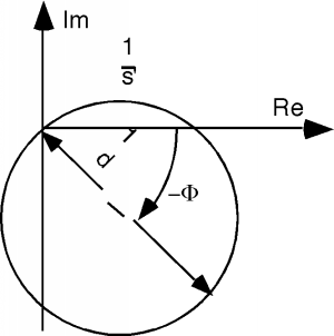
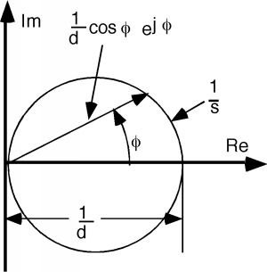Figure \(\PageIndex{4}\): A plot of 1/s

A careful look at Figure \(\PageIndex{4}\) should allow you to convince yourself that Equation is an equation for a circle on the complex plane, with a diameter $\frac{1}{d}$. If $s$ is not parallel to the imaginary axis, but rather has its perpendicular to the origin at some angle $$φφ, to make a line $s^{\prime }$ as shown in Figure \(\PageIndex{5}\). Since $s^{\prime }=s{e}^{i\phi }$, taking $\frac{1}{s}$ simply will give us a circle with a diameter of $\frac{1}{d}$, which has been rotated by an angle $$φφ from the real axis as shown in Figure \(\PageIndex{6}\). And so we come to the one fact we have to keep in mind: "The inverse of a straight line on the complex plane is a circle, whose diameter is the inverse of the distance between the line and the origin."

Figure \(\PageIndex{5}\): The Line s' is the line $s$ multiplied by \(e^{i \phi}\)

Figure \(\PageIndex{6}\): Inverse of a rotated line