6.8: The Smith Chart

Last updated
Save as PDF

Page ID: 88580

$ \newcommand{\vecs}[1]{\overset { \scriptstyle \rightharpoonup} {\mathbf{#1}} } $ $ \newcommand{\vecd}[1]{\overset{-\!-\!\rightharpoonup}{\vphantom{a}\smash {#1}}} $$\newcommand{\id}{\mathrm{id}}$ $ \newcommand{\Span}{\mathrm{span}}$ $ \newcommand{\kernel}{\mathrm{null}\,}$ $ \newcommand{\range}{\mathrm{range}\,}$ $ \newcommand{\RealPart}{\mathrm{Re}}$ $ \newcommand{\ImaginaryPart}{\mathrm{Im}}$ $ \newcommand{\Argument}{\mathrm{Arg}}$ $ \newcommand{\norm}[1]{\| #1 \|}$ $ \newcommand{\inner}[2]{\langle #1, #2 \rangle}$ $ \newcommand{\Span}{\mathrm{span}}$ $\newcommand{\id}{\mathrm{id}}$ $ \newcommand{\Span}{\mathrm{span}}$ $ \newcommand{\kernel}{\mathrm{null}\,}$ $ \newcommand{\range}{\mathrm{range}\,}$ $ \newcommand{\RealPart}{\mathrm{Re}}$ $ \newcommand{\ImaginaryPart}{\mathrm{Im}}$ $ \newcommand{\Argument}{\mathrm{Arg}}$ $ \newcommand{\norm}[1]{\| #1 \|}$ $ \newcommand{\inner}[2]{\langle #1, #2 \rangle}$ $ \newcommand{\Span}{\mathrm{span}}$$\newcommand{\AA}{\unicode[.8,0]{x212B}}$

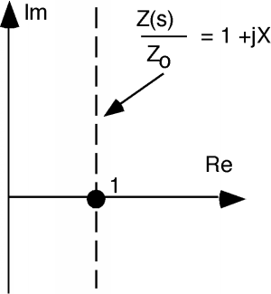
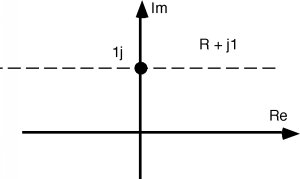
Now let's see how we can use The Bilinear Transform to get the coordinates on the $\frac{Z (s)}{Z_{0}}$ plane transferred over onto the $r (s)$ plane. The Bilinear Transform tells us how to take any $\frac{Z (s)}{Z_{0}}$ and generate an $r (s)$ from it. Let's start with an easy one. We will assume that $\frac{Z (s)}{Z_{0}} = 1 + i X$ , which is a vertical line that passes through 1 and can take on whatever imaginary part it wants, as shown in Figure $\PageIndex{1}$.

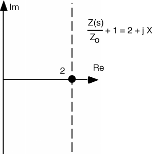
The complex plane with a vertical dotted line passing through the point with value 1 on the real axis. The line describes Z(s) divided by Z_0, which has a value of 1 + jX. — Figure $\PageIndex{1}$: Complex Impedence With Real Part = +1

According to The Bilinear Transform, the first thing we should do is add 1 to $\frac{Z (s)}{Z_{0}}$ . This gives us the line $2 + i X$ Figure $\PageIndex{2}$.

A complex plane with a vertical line passing through the point of value 2 on the real axis. The line describes Z(s) divided by Z_0, plus 1. This equals 2 + jX. — Figure $\PageIndex{2}$: Adding 1

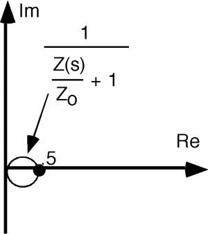
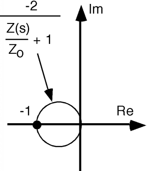
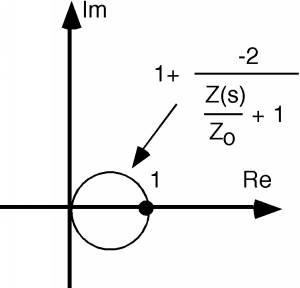
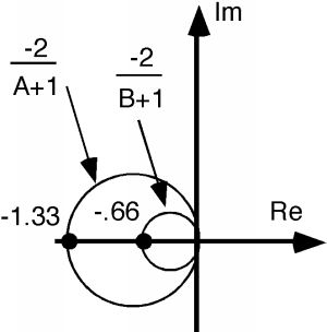
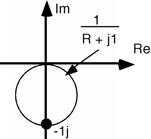
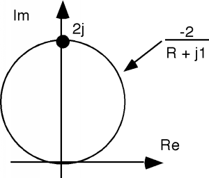
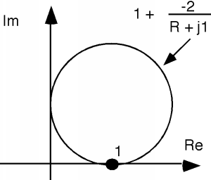
Now, we take the inverse of this, which will give us a circle of diameter 1/2 as shown in Figure $\PageIndex{3}$. Now, according to The Bilinear Transform we take this circle and multiply it by -2, which is shown in Figure $\PageIndex{4}$.

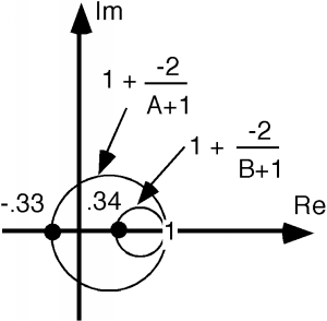
The inverse of 1 plus the quotient of Z(s) and Z_0 is a circle of diameter 0.5. The circle is centered on the real axis, with its leftmost point lying on the origin. — Figure $\PageIndex{3}$: Inverting the line

The expression from Figure 3 above is multiplied by -2. The corresponding graph on the complex plane is a circle of diameter 1, centered on the real axis and with its rightmost point lying at the origin. — Figure $\PageIndex{4}$: Multiplying by -2

And finally, we take the circle and add +1 to it as shown in Figure $\PageIndex{5}$. There, we are done with the transform. The vertical line on the $\frac{Z (s)}{Z_{0}}$ plane that represents an impedance with a real part of +1 and an imaginary part with any value from $- (i \infty)$ to $i \infty$ has been reduced to a circle with diameter 1, passing through $0$ and $1$ on the complex $r (s)$ plane.

The value of 1 is added to the expression from Figure 4 above. The corresponding graph on the complex plane is a circle of diameter 1, centered on the real axis with its leftmost point lying at the origin. — Figure $\PageIndex{5}$: Adding 1 once again

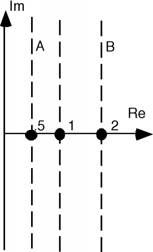
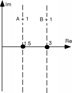
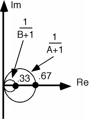
Let's do the same thing for $\frac{Z (s)}{Z_{0}} = 0.5 + i X$ and $\frac{Z (s)}{Z_{0}} = 2 + i X$ . We'll call these lines A and B respectively and just add these to the sketches we already have, as shown in Figure $\PageIndex{6}$. Follow along with The Bilinear Transform, and see if you can figure out where each of these sketches comes from. We will simply be doing the same things again: add 1, invert, multiply by -2, and add 1 once again. As you can see in Figures $\PageIndex{7}$, $\PageIndex{8}$, $\PageIndex{9}$, and $\PageIndex{10}$, we get more circles. For lines inside the +1 real part, we end up with a circle that is larger than the +1 circle, and for lines which have a real part greater than +1, we end up with circles which are smaller in diameter than the +1 circle. All circles pass through the +1 point on the $r (s)$ plane and are tangent to one another.

A complex plane containing three vertical lines. One line passes through the point 0.5 on the real axis, and is labeled A. The second line passes through the point 1 on the real axis. The third line passes through the point 2 on the real axis and is labeled B. — Figure $\PageIndex{6}$: Two more examples

Complex plane containing two vertical lines. One of the lines, passing through point 1.5 on the real axis, is the equation of A+1. The other line, passing through point 3 on the real axis, is the equation of B+1. — Figure $\PageIndex{7}$: Add +1 to each

Complex plane containing the graph of the inverse of A+1, which takes the form of a circle of radius 2/3 centered on the real axis with its leftmost point at the origin; and the graph of the inverse of B+1, which takes the form of a circle of radius 1/3 with its leftmost point at the origin. — Figure $\PageIndex{8}$: Inverting

Complex plane containing the graph of -2 times the inverse of A+1, which takes the form of a circle of radius 4/3 centered on the real axis with its rightmost point at the origin; and the graph of -2 times the inverse of B+1, which takes the form of a circle of radius 2/3 with its rightmost point at the origin. — Figure $\PageIndex{9}$: Multiply by -2

A complex plane containing graphs of 1 plus each of the expressions from Figure 9 above. The shapes and sizes of the circular graphs remain the same, but both of their positions are shifted to the right by a distance of 1. — Figure $\PageIndex{10}$: The Final Result

There are two special lines we should worry about. One is $\frac{Z (s)}{Z_{0}} = i X$ , the imaginary axis. We will put all of the transform steps together on Figure $\PageIndex{11}$. We start on the axis, shift over one, get a circle with unity diameter when we invert, grow by two and flip around the imaginary axis when we multiply by -2, and then hop one to the right when +1 is added. Once again, you should work your way through the various steps to make sure you have a good understanding as to how this procedure is supposed to happen. Note that even the imaginary axis on the $\frac{Z (s)}{Z_{0}}$ plane gets transformed into a circle when we go over onto the $r (s)$ plane.

A complex plane with a vertical line jX on the imaginary axis. A vertical line that passes through the point 1 on the real axis is jX + 1. The inverse of this line is a circle of diameter 1, centered on the real axis with its leftmost point at the origin. The graph of -2 times this expression is a circle of diameter 2, centered on the real axis with its rightmost point at the origin. The graph of 1 plus this expression is a circle of diameter 2, centered at the origin. — Figure $\PageIndex{11}$: Another transform, which transforms $i X$ to the $r (s)$ plane.

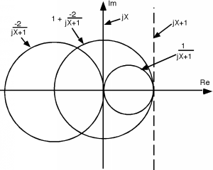
The other line we should worry about is $\frac{Z (s)}{Z_{0}} = \infty + i X$ . Now $\infty + 1 = \infty$ , and $\frac{-2}{\infty} = 0.0 + 1 = 1$ , and so the line $1 + i X$ gets mapped into a point at 1 when we do our transformation onto the $r (s)$ plane. Even points at $\infty$ on the $\frac{Z (s)}{Z_{0}}$ plane end up on the $r (s)$ plane, and are easily accessible!

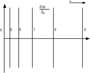
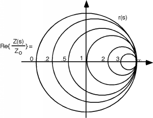
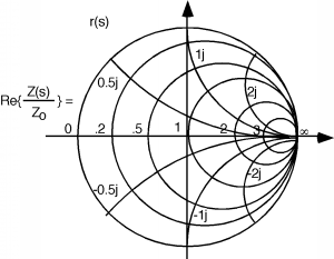
OK, Figure $\PageIndex{12}$ is a plot of the $\frac{Z (s)}{Z_{0}}$ plane. The lines shown represent the real part of $\frac{Z (s)}{Z_{0}}$ that we want to transform. We run them all through The Bilinear Transform, to get them onto the $r (s)$ plane. Now we have a whole family of circles, the biggest of which has a diameter of 2 (which corresponds to the imaginary axis) and the smallest of which has a diameter of 0 (which corresponds to points at $\infty$ ) Figure $\PageIndex{13}$. The circles all fit within one another, and since a +1 was added to every transform as the final bit of manipulation, all of the circles pass through the point +1, $0 i$ . Circles with smaller diameters correspond to larger values of real $\frac{Z (s)}{Z_{0}}$ , while the larger circles correspond to the lesser values of $\frac{Z (s)}{Z_{0}}$ .

Plane of the quotient of Z(s) and Z_0, containing 5 vertical lines. From left to right, they represent values of 0.2, 0.5, 1, 2, and 3. — Figure $\PageIndex{12}$: Adding other constant real part line to the $\frac{Z (s)}{Z_{0}}$ plane.

Graphs on the r(s) plane of all the lines from Figure 12 above, run through the bilinear transform. This corresponds to the real component of Z(s) over Z_0. Each takes the form of a circle centered on the horizontal axis, with its rightmost point at the value of 1 on the horizontal axis. Larger values of the original lines translate to smaller radii, and smaller values of the original lines translate to larger radii. — Figure $\PageIndex{13}$: Family of circles, which is a family of $ℜ (\frac{Z (s)}{Z_{0}})$

Well, we're halfway there. Now all we have to do is find the transform for the coordinate lines which correspond to the imaginary part of $\frac{Z (s)}{Z_{0}}$ . Let's look at $\frac{Z (s)}{Z_{0}} = R + i 1$ . When we add +1 to this, nothing happens! The line just slides over 1 unit, and looks just the same, as in Figure $\PageIndex{14}$. Now we take its inverse. This will gives us a circle, but since the line we are inverting lies at an angle of $90^{°}$ with respect to the real axis, the major diameter of the circle will lie at an angle of $- 90^{°}$ when we go through the inversion process. This gives us a circle which is lying in the $- i$ region of the complex plane Figure.

Complex plane containing a horizontal line that passes through the point 1j on the imaginary axis. Equation of the line is given as R + j1. — Figure $\PageIndex{14}$: A line of constant imaginary part

Complex plane showing the graph of the inverse of R + j1. The graph takes the form of a circle with its top at the origin and its bottom at the point -1j on the imaginary axis. — Figure $\PageIndex{15}$: After inverting

The next thing we do is to take this circle and multiply by -2. This will make the circle twice as large, but will also reflect it back up into the $i$ region of the complex plane, as shown in Figure $\PageIndex{16}$.

Complex plane showing the graph of -2 times the inverse of R + j1. Graph takes the form of a circle with its top at point 2j on the imaginary axis and its bottom at the origin. — Figure $\PageIndex{16}$: Multiply by -2...

And, finally, we add 1 to it, which causes the circle to hop one over to the right (Figure $\PageIndex{17}$).

Complex plane containing the graph of 1 added to the equation from Figure 16 above. Graph takes the form of the circle from Figure 16 shifted 1 to the right, so its bottom is now located at the point 1 on the real axis. — Figure $\PageIndex{17}$: ...and add 1

We can do the same thing to other lines of constant imaginary part and we can then add more circles. (Or partial circles, for it makes no sense to go beyond the $ℜ (\frac{Z (s)}{Z_{0}}) = 0$ circles, as beyond that is the region corresponding to negative real part, which we would not expect to encounter in most transmission lines.) Take at least one of the other circles drawn here in Figure $\PageIndex{18}$ and see if you can get it to end up in about the right place.

he real portion of Z(s)/Z_0, which has a range of 0 to positive infinity, is represented on the r(s) plane by circles centered on the horizontal axis, with their rightmost points all at point (1, 0). The imaginary portion is shown by partial circles that end at the borders of the largest circle representing a real value that is shown. Positive imaginary values correspond to circles above the horizontal axis, with their lowest point at (1, 0), and negative imaginary values correspond to circles below the horizontal axis with their lowest point at (1, 0). For all circles, the diameters decrease as the magnitude of the value they represent increases. The maximum possible radius is 1, corresponding to a value of 0. — Figure $\PageIndex{18}$: The complete transformation

There is one line of interest which we have a take a little care with. That is the real axis, $\frac{Z (s)}{Z_{0}} = 0 + i X$ . This line is a distance 0 away from the origin, and so when we invert it, we get a circle with $\infty$ diameter. That's OK though, because that is just a straight line. So, the real axis of the $\frac{Z (s)}{Z_{0}}$ plane transforms into the real axis on the $r (s)$ plane.

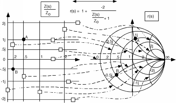
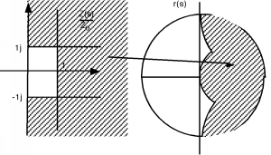
We have done a most wondrous thing! (Although you may not realize it yet.) We have taken the entire half plane of complex impedance $\frac{Z (s)}{Z_{0}}$ and mapped the whole thing into a circle with diameter 1! Let's put the two of them side by side. (Although we can't show the whole $\frac{Z (s)}{Z_{0}}$ plane of course.) These are shown in Figure $\PageIndex{19}$, where we show how each line on $\frac{Z (s)}{Z_{0}}$ maps into a (curved) line on the $r (s)$ plane. Note also, that for every point on the $\frac{Z (s)}{Z_{0}}$ plane ("A" and "B") there is a corresponding point on the $r (s)$ plane. Pick a couple more points, "C" and "D" and locate them either on the $\frac{Z (s)}{Z_{0}}$ plane, or the $r (s)$ plane, and then find the corresponding point on the other plane.

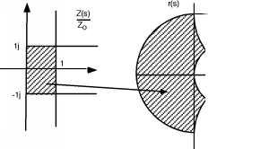
Mapping of points of Z(s)/Z_0 on the complex plane to the corresponding points on the r(s) plane. A point at a given real-component value and imaginary-component value on the complex plane is located at the intersection of the circles representing that real-component value and imaginary-component value on the r(s) plane. — Figure $\PageIndex{19}$: The mapping

Note that the mapping is not very uniform. All of the region where either the real or imaginary part of $\frac{Z (s)}{Z_{0}}$ is $1$ (a small square on $\frac{Z (s)}{Z_{0}}$ maps into a major fraction of the $r (s)$ plane as shown in Figure $\PageIndex{20}$ whereas all the rest of the $\frac{Z (s)}{Z_{0}}$ plane, all the way out to infinity in three directions ( $\infty$ , $i \infty$ , and $- (i \infty)$ ) map into the rest of the $r (s)$ circle as shown in Figure $\PageIndex{21}$.

The rectangle on the complex plane bounded by the imaginary axis, Re=1, Im=1j, and Im=-1j maps to a region on the r(s) plane that consists of the semicircle with radius 1 to the left of the vertical axis, as well as a small portion of the region to the right of that axis. — Figure $\PageIndex{20}$: Mapping 1, $1 i$

The region of the complex plane to the right of the imaginary axis and outside of the rectangle discussed in Figure 20 above maps to an r(s) region consisting of less than half of the semicircle, which is the part not covered in Figure 20. — Figure $\PageIndex{21}$: Mapping the rest

This graph or transformation is called a Smith Chart, after the Bell Labs worker who first thought it up. It is a most useful and powerful graphical solution to the transmission line problem. In Introduction to Using the Smith Chart we will spend a little time seeing how and why it can be so useful.