6.9: Introduction to Using the Smith Chart

Last updated
Save as PDF

Page ID: 88581

$ \newcommand{\vecs}[1]{\overset { \scriptstyle \rightharpoonup} {\mathbf{#1}} } $

$ \newcommand{\vecd}[1]{\overset{-\!-\!\rightharpoonup}{\vphantom{a}\smash {#1}}} $

$ \newcommand{\id}{\mathrm{id}}$ $ \newcommand{\Span}{\mathrm{span}}$

( \newcommand{\kernel}{\mathrm{null}\,}\) $ \newcommand{\range}{\mathrm{range}\,}$

$ \newcommand{\RealPart}{\mathrm{Re}}$ $ \newcommand{\ImaginaryPart}{\mathrm{Im}}$

$ \newcommand{\Argument}{\mathrm{Arg}}$ $ \newcommand{\norm}[1]{\| #1 \|}$

$ \newcommand{\inner}[2]{\langle #1, #2 \rangle}$

$ \newcommand{\Span}{\mathrm{span}}$

$ \newcommand{\id}{\mathrm{id}}$

$ \newcommand{\Span}{\mathrm{span}}$

$ \newcommand{\kernel}{\mathrm{null}\,}$

$ \newcommand{\range}{\mathrm{range}\,}$

$ \newcommand{\RealPart}{\mathrm{Re}}$

$ \newcommand{\ImaginaryPart}{\mathrm{Im}}$

$ \newcommand{\Argument}{\mathrm{Arg}}$

$ \newcommand{\norm}[1]{\| #1 \|}$

$ \newcommand{\inner}[2]{\langle #1, #2 \rangle}$

$ \newcommand{\Span}{\mathrm{span}}$ $ \newcommand{\AA}{\unicode[.8,0]{x212B}}$

$ \newcommand{\vectorA}[1]{\vec{#1}} % arrow$

$ \newcommand{\vectorAt}[1]{\vec{\text{#1}}} % arrow$

$ \newcommand{\vectorB}[1]{\overset { \scriptstyle \rightharpoonup} {\mathbf{#1}} } $

$ \newcommand{\vectorC}[1]{\textbf{#1}} $

$ \newcommand{\vectorD}[1]{\overrightarrow{#1}} $

$ \newcommand{\vectorDt}[1]{\overrightarrow{\text{#1}}} $

$ \newcommand{\vectE}[1]{\overset{-\!-\!\rightharpoonup}{\vphantom{a}\smash{\mathbf {#1}}}} $

$ \newcommand{\vecs}[1]{\overset { \scriptstyle \rightharpoonup} {\mathbf{#1}} } $

$ \newcommand{\vecd}[1]{\overset{-\!-\!\rightharpoonup}{\vphantom{a}\smash {#1}}} $

$\newcommand{\avec}{\mathbf a}$ $\newcommand{\bvec}{\mathbf b}$ $\newcommand{\cvec}{\mathbf c}$ $\newcommand{\dvec}{\mathbf d}$ $\newcommand{\dtil}{\widetilde{\mathbf d}}$ $\newcommand{\evec}{\mathbf e}$ $\newcommand{\fvec}{\mathbf f}$ $\newcommand{\nvec}{\mathbf n}$ $\newcommand{\pvec}{\mathbf p}$ $\newcommand{\qvec}{\mathbf q}$ $\newcommand{\svec}{\mathbf s}$ $\newcommand{\tvec}{\mathbf t}$ $\newcommand{\uvec}{\mathbf u}$ $\newcommand{\vvec}{\mathbf v}$ $\newcommand{\wvec}{\mathbf w}$ $\newcommand{\xvec}{\mathbf x}$ $\newcommand{\yvec}{\mathbf y}$ $\newcommand{\zvec}{\mathbf z}$ $\newcommand{\rvec}{\mathbf r}$ $\newcommand{\mvec}{\mathbf m}$ $\newcommand{\zerovec}{\mathbf 0}$ $\newcommand{\onevec}{\mathbf 1}$ $\newcommand{\real}{\mathbb R}$ $\newcommand{\twovec}[2]{\left[\begin{array}{r}#1 \\ #2 \end{array}\right]}$ $\newcommand{\ctwovec}[2]{\left[\begin{array}{c}#1 \\ #2 \end{array}\right]}$ $\newcommand{\threevec}[3]{\left[\begin{array}{r}#1 \\ #2 \\ #3 \end{array}\right]}$ $\newcommand{\cthreevec}[3]{\left[\begin{array}{c}#1 \\ #2 \\ #3 \end{array}\right]}$ $\newcommand{\fourvec}[4]{\left[\begin{array}{r}#1 \\ #2 \\ #3 \\ #4 \end{array}\right]}$ $\newcommand{\cfourvec}[4]{\left[\begin{array}{c}#1 \\ #2 \\ #3 \\ #4 \end{array}\right]}$ $\newcommand{\fivevec}[5]{\left[\begin{array}{r}#1 \\ #2 \\ #3 \\ #4 \\ #5 \\ \end{array}\right]}$ $\newcommand{\cfivevec}[5]{\left[\begin{array}{c}#1 \\ #2 \\ #3 \\ #4 \\ #5 \\ \end{array}\right]}$ $\newcommand{\mattwo}[4]{\left[\begin{array}{rr}#1 \amp #2 \\ #3 \amp #4 \\ \end{array}\right]}$ $\newcommand{\laspan}[1]{\text{Span}\{#1\}}$ $\newcommand{\bcal}{\cal B}$ $\newcommand{\ccal}{\cal C}$ $\newcommand{\scal}{\cal S}$ $\newcommand{\wcal}{\cal W}$ $\newcommand{\ecal}{\cal E}$ $\newcommand{\coords}[2]{\left\{#1\right\}_{#2}}$ $\newcommand{\gray}[1]{\color{gray}{#1}}$ $\newcommand{\lgray}[1]{\color{lightgray}{#1}}$ $\newcommand{\rank}{\operatorname{rank}}$ $\newcommand{\row}{\text{Row}}$ $\newcommand{\col}{\text{Col}}$ $\renewcommand{\row}{\text{Row}}$ $\newcommand{\nul}{\text{Nul}}$ $\newcommand{\var}{\text{Var}}$ $\newcommand{\corr}{\text{corr}}$ $\newcommand{\len}[1]{\left|#1\right|}$ $\newcommand{\bbar}{\overline{\bvec}}$ $\newcommand{\bhat}{\widehat{\bvec}}$ $\newcommand{\bperp}{\bvec^\perp}$ $\newcommand{\xhat}{\widehat{\xvec}}$ $\newcommand{\vhat}{\widehat{\vvec}}$ $\newcommand{\uhat}{\widehat{\uvec}}$ $\newcommand{\what}{\widehat{\wvec}}$ $\newcommand{\Sighat}{\widehat{\Sigma}}$ $\newcommand{\lt}{<}$ $\newcommand{\gt}{>}$ $\newcommand{\amp}{&}$ $\definecolor{fillinmathshade}{gray}{0.9}$

Now that we know what it is, we will investigate some of the application and uses of the Smith Chart. For the text, we will use my new "mini Smith Chart," which is reproduced below. Clearly, there is not much detail here, and our answers will not be as accurate as they would be if we used a full-size chart, but we want to get ideas across here, not the best number possible, and with the small size, we won't run out of paper before everything is done.

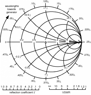
A version of the Smith Chart showing circles corresponding to real values of 0, 0.2, 0.5, 1, 2, and 4, and circles corresponding to imaginary values of positive and negative 0.2j, 0.5j, 1j, and 2j. The intersections of the imaginary-value circles with the outermost real-valued circle are marked as fractions of lambda or wavelength: 0 at the leftmost point of the outer circle, increasing in the clockwise direction so that a full rotation corresponds to 0.5 lambda. Scales for the VSWR and the reflection coefficient Gamma are located below the chart. — Figure $\PageIndex{1}$: The Smith Chart

Note that we have a couple of "extras" on the chart. The two scales at the bottom of the chart can be used to either set or measure radial variables such as the magnitude of the reflection coefficient $| Γ |$ , or the VSWR, as it turns out that in practice, what one can actually measure on a line is the VSWR. Remember, there is a direct relationship between the VSWR and the magnitude of the reflection coefficient.

VSWR = \frac{1 + | Γ |}{1 - | Γ |}

| Γ | = \frac{VSWR - 1}{VSWR + 1}

Since $| r (s) | = | Γ |$ , once we have the VSWR, we have $| r (s) |$ and so we know how big a circle we need on the Smith Chart in order to go from one place to the next. Note also that there is a scale around the outside of the chart which is given in fractions of a wavelength. Since $r (s)$ rotates around at a rate $2 β s$ and $β = \frac{2}{π}$ , we could either show distance in centimeters or something and then change the scale whenever we change wavelength, or we could just use a distance scale in $λ$ and measure all distances in units of the wavelength. This is what we shall do. Since the rate of rotation is $2 β s$ , one trip around the Smith Chart is the same as going one-half of a wavelength down the line. Rotation in a clockwise direction is the same as moving away from the load towards the generator, while motion along the line in the other direction (towards the load) calls for counterclockwise rotation. The scale is, of course, a relative one, and so we will have to re-set our zero, depending upon where the load, etc. are really located. This will all become clearer as we do an example.

Let's start out with the simplest thing we can, with just a generator, line and load, as shown in Figure $\PageIndex{2}$. Our task will be to find the input impedance, $Z_{in}$ , for the line, so that we can figure the input voltage.

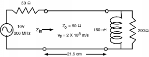
A transmission line with an impedance of Z_0 50 Ohms, v_p of 2 times 10^8 m/s, and length 21.5 cm has its left end attached to a sinusoidal 10V voltage source of frequency 200 MHz and source resistance 50 Ohms, and its right end attached to a 160-nH inductor and a 200-Ohm resistor in parallel. — Figure $\PageIndex{2}$: Transmission line problem

For this first problem, we are going to start out with all the basics. In later examples, we probably will only give lengths in wavelengths, and impedances in terms of $Z_{0}$ , but let's do this the whole way through.

Search

Text Color

Text Size

Margin Size

Font Type