6.10: Simple Calculations with the Smith Chart

So, what do we do for \(Z_{L}\)? A quick glance at a transmission line problem shows that at the load we have a resistor and an inductor in parallel. This was done on purpose, to show you one of the powerful aspects of the Smith Chart. Based on what you know from circuit theory, you would calculate the load impedance by using the formula for two impedances in parallel, \(Z_{L} = \frac{i \omega LR}{i \omega L + R}\), which will be somewhat messy to calculate.

Let's remember the formula for what the Smith Chart represents in terms of the phasor \(r(s)\). \[\frac{Z_{L}}{Z_{0}} = \frac{1 + r(s)}{1 - r(s)}\]

Let's invert this expression: \[\begin{array}{l} \dfrac{Z_{L}}{Z_{0}} &=& \dfrac{\frac{1}{Z_{L}}}{\frac{1}{Z_{0}}} \\[4pt] &=& \dfrac{Y_{L}}{Y_{0}} \\[4pt] &=& \dfrac{1 - r(s)}{1 + r(s)} \end{array}\]

Equation \(\PageIndex{3}\) says that is we want to get an admittance instead of an impedance, all we have to do is substitute \(-r(s)\) for \(r(s)\) on the Smith Chart plane! In our case, \[Y_{0} = \frac{1}{Z_{0}} = \frac{1}{50} = 0.02\]

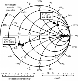
We have two elements in parallel for the load (\(Y_{L} = Y + iB\)), so we can easily add their admittances, normalize them to \(Y_{0}\), put them on the Smith Chart, go \(180^{\circ}\) around (same thing as letting \(-r(s) = r(s)\)) and read off \(\frac{Z_{L}}{Z_{0}}\). For a \(200 \mathrm{~\Omega}\) resistor, the conductance \(G\) equals \(\frac{1}{200} = 0.005\). \(Y_{0} = 0.02\) so \(\frac{G}{Y_{0}} = 0.25\). The generator is operating at a frequency of \(200 \mathrm{~MHz}\) so \(\omega = 2 \pi f = 1.25 \times 10^{9} \mathrm{~s}^{-1}\) and the inductor has a value of \(160 \mathrm{~nH}\), so \(i \omega L = 200i\) and \(B = \frac{1}{i \omega L} = -0.005i\) and \(\frac{B}{Y_{0}} = -0.25i\).

We plot this on the Smith Chart by first finding the circle that corresponds to a real part of \(0.25\), and then we go down onto the lower half of the chart since that is where all the negative reactive parts are, and we find the curve which represents \(-0.25i\). Where these curves intersect, we put a dot, and mark the location as \(\frac{Y_{L}}{Y_{0}}\). Now to find \(\frac{Z_{L}}{Z_{0}}\), we simply reflect half way around to the opposite side of the chart, which happens to be about \(\frac{Y_{L}}{Y_{0}} = 2 + 2i\), and we mark that as well. Note that we can take the length of the line from the center of the Smith Chart to our \(\frac{Z_{L}}{Z_{0}}\) and move it down to the \(|\Gamma|\) scale and find that the reflection coefficient has a magnitude of about \(0.6\). On a real Smith Chart, there is also a phase angle scale on the outside of the circle (where our distance scale is) which you can use to read off the phase angle of the reflection coefficient as well. Putting that scale on the "mini Smith Chart" would clog things up too much, but the phase angle of \(\Gamma\) is about \(3.0^{\circ}\).

Figure \(\PageIndex{1}\): Moving down the transmission line

Now the wavelength of the signal on the line is given as \[\begin{array}{l} \lambda &=& \dfrac{\nu}{f} \\[4pt] &=& \dfrac{2.8 \times 10^{8}}{200 \times 10^{6}} \\[4pt] &=& 1 \mathrm{~m} \end{array}\]

The input to the line is located \(21.5 \mathrm{~cm}\) or \(0.215 \ \lambda\) away from the load. Thus, we start at \(\frac{Z_{L}}{Z_{0}}\), and rotate around on a circle of constant radius a distance \(0.215 \ \lambda\) towards the generator. To do this, we extend a line out from our \(\frac{Z_{L}}{Z_{0}}\) point to the scale and read a relative distance of \(0.208 \ \lambda\). We add \(0.215 \ \lambda\) to this, and get \(0.423 \ \lambda\). Thus, if we rotate around the Smith Chart, on our circle of constant radius since after all, all we are doing is following \(r(s)\) as it rotates around from the load to the input to the line, when we get to \(0.423 \ \lambda\) we stop, draw a line out from the center, and where it intercepts the circle, we read off \(\frac{Z_{L}}{Z_{0}}\) from the grid lines on the Smith Chart. We find that

Figure \(\PageIndex{2}\): Using a Smith Chart to convert from admittance to impedance

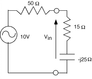
Thus, \(Z_{\text{in}} = 15 + -25i\) ohms in Figure \(\PageIndex{3}\). Or, the impedance at the input to the line looks like a \(15 \ \Omega\) resistor in series with a capacitor whose reactance \(iX = -25i\), or, since \(X_{\text{cap}} = \frac{1}{i \omega C}\), we find that \[\begin{array}{l} C &=& \dfrac{1}{2 \pi 200 \times 200 \times 10^{6}} \\[4pt] &=& 31.8 \mathrm{~pF} \end{array}\]

To find \(V_{\text{in}}\), there is no avoiding doing some complex math: \[V_{\text{in}} = \frac{15 + -25i}{50 + 15 + -25i} 10\]

which we write in polar notation, divide, figure the voltage and then return to rectangular notation. \[V_{\text{in}} = \frac{29.1 \angle 59}{69.6 \angle -21} 10\] \[\begin{array}{l} V_{\text{in}} &=& 0.418 \angle -38 \times 10 \\ &=& 4.18 \angle -38 \\ &=& 3.30 + -2.58i \end{array}\]

Figure \(\PageIndex{3}\): Find \(V_{\text{in}}\)

If at this point we needed to find the actual voltage phasor \(V^{+}\) we would have to use the equation \[\begin{array}{l} V_{\text{in}} &=& V^{+} e^{i \beta L} + \Gamma V^{+} e^{-(i \beta L)} \\ &=& V^{+} e^{i \beta L} + |\Gamma| V^{+} e^{i(\theta_{r} - \beta L)} \end{array}\]

where \(\beta = \frac{2 \pi}{L}\) is the propagation constant for the line as mentioned in a previous section, and \(L\) is the length of the line.

For this example, \(\beta L = \frac{2 pi}{\lambda}\), \(0.215 \lambda = 1.35 \mathrm{~radians}\), and \(\theta_{\Gamma} = \Gamma = 0.52 \mathrm{~radians}\). Thus we have: \[V_{\text{in}} = V^{+} e^{i 1.35} + 0.52 V^{+} e^{i(0.52 - 1.35)}\]

which then gives us: \[V^{+} = \frac{V_{\text{in}}}{e^{i 1.35} + 0.52 e^{i(0.52 - 1.35)}}\]

When you expand the exponentials, add and combine in rectangular coordinates, change to polar, and divide, you will get a phasor value for \(V^{+}\). If you do it correctly, you will find that \(V^{+} = 5.04 \angle -71.59\).

Many times we don't care about \(V^{+}\) itself, but are more interested in how much power is being delivered to the load. Note that power delivered to the input of the line is also the amount of power which is delivered to the load! Finding \(I_{\text{in}}\) is easy, it's just \(\frac{V_{\text{in}}}{Z_{\text{in}}}\). All we have to do is change \(Z_{\text{in}}\) to polar form. \[\begin{array}{l} Z_{\text{in}} &=& 15 + -25i \\ &=& 29.1 \angle 59 \end{array}\] \[\begin{array}{l} I_{\text{in}} &=& \dfrac{V_{\text{in}}}{Z_{\text{in}}} \\ &=& \frac{4.18 \angle 38}{29.1 \angle 59} \\ &=& 0.144 \angle 21 \end{array}\]