6.12: Finding ZL
- Page ID
- 88584
\( \newcommand{\vecs}[1]{\overset { \scriptstyle \rightharpoonup} {\mathbf{#1}} } \)
\( \newcommand{\vecd}[1]{\overset{-\!-\!\rightharpoonup}{\vphantom{a}\smash {#1}}} \)
\( \newcommand{\id}{\mathrm{id}}\) \( \newcommand{\Span}{\mathrm{span}}\)
( \newcommand{\kernel}{\mathrm{null}\,}\) \( \newcommand{\range}{\mathrm{range}\,}\)
\( \newcommand{\RealPart}{\mathrm{Re}}\) \( \newcommand{\ImaginaryPart}{\mathrm{Im}}\)
\( \newcommand{\Argument}{\mathrm{Arg}}\) \( \newcommand{\norm}[1]{\| #1 \|}\)
\( \newcommand{\inner}[2]{\langle #1, #2 \rangle}\)
\( \newcommand{\Span}{\mathrm{span}}\)
\( \newcommand{\id}{\mathrm{id}}\)
\( \newcommand{\Span}{\mathrm{span}}\)
\( \newcommand{\kernel}{\mathrm{null}\,}\)
\( \newcommand{\range}{\mathrm{range}\,}\)
\( \newcommand{\RealPart}{\mathrm{Re}}\)
\( \newcommand{\ImaginaryPart}{\mathrm{Im}}\)
\( \newcommand{\Argument}{\mathrm{Arg}}\)
\( \newcommand{\norm}[1]{\| #1 \|}\)
\( \newcommand{\inner}[2]{\langle #1, #2 \rangle}\)
\( \newcommand{\Span}{\mathrm{span}}\) \( \newcommand{\AA}{\unicode[.8,0]{x212B}}\)
\( \newcommand{\vectorA}[1]{\vec{#1}} % arrow\)
\( \newcommand{\vectorAt}[1]{\vec{\text{#1}}} % arrow\)
\( \newcommand{\vectorB}[1]{\overset { \scriptstyle \rightharpoonup} {\mathbf{#1}} } \)
\( \newcommand{\vectorC}[1]{\textbf{#1}} \)
\( \newcommand{\vectorD}[1]{\overrightarrow{#1}} \)
\( \newcommand{\vectorDt}[1]{\overrightarrow{\text{#1}}} \)
\( \newcommand{\vectE}[1]{\overset{-\!-\!\rightharpoonup}{\vphantom{a}\smash{\mathbf {#1}}}} \)
\( \newcommand{\vecs}[1]{\overset { \scriptstyle \rightharpoonup} {\mathbf{#1}} } \)
\( \newcommand{\vecd}[1]{\overset{-\!-\!\rightharpoonup}{\vphantom{a}\smash {#1}}} \)
\(\newcommand{\avec}{\mathbf a}\) \(\newcommand{\bvec}{\mathbf b}\) \(\newcommand{\cvec}{\mathbf c}\) \(\newcommand{\dvec}{\mathbf d}\) \(\newcommand{\dtil}{\widetilde{\mathbf d}}\) \(\newcommand{\evec}{\mathbf e}\) \(\newcommand{\fvec}{\mathbf f}\) \(\newcommand{\nvec}{\mathbf n}\) \(\newcommand{\pvec}{\mathbf p}\) \(\newcommand{\qvec}{\mathbf q}\) \(\newcommand{\svec}{\mathbf s}\) \(\newcommand{\tvec}{\mathbf t}\) \(\newcommand{\uvec}{\mathbf u}\) \(\newcommand{\vvec}{\mathbf v}\) \(\newcommand{\wvec}{\mathbf w}\) \(\newcommand{\xvec}{\mathbf x}\) \(\newcommand{\yvec}{\mathbf y}\) \(\newcommand{\zvec}{\mathbf z}\) \(\newcommand{\rvec}{\mathbf r}\) \(\newcommand{\mvec}{\mathbf m}\) \(\newcommand{\zerovec}{\mathbf 0}\) \(\newcommand{\onevec}{\mathbf 1}\) \(\newcommand{\real}{\mathbb R}\) \(\newcommand{\twovec}[2]{\left[\begin{array}{r}#1 \\ #2 \end{array}\right]}\) \(\newcommand{\ctwovec}[2]{\left[\begin{array}{c}#1 \\ #2 \end{array}\right]}\) \(\newcommand{\threevec}[3]{\left[\begin{array}{r}#1 \\ #2 \\ #3 \end{array}\right]}\) \(\newcommand{\cthreevec}[3]{\left[\begin{array}{c}#1 \\ #2 \\ #3 \end{array}\right]}\) \(\newcommand{\fourvec}[4]{\left[\begin{array}{r}#1 \\ #2 \\ #3 \\ #4 \end{array}\right]}\) \(\newcommand{\cfourvec}[4]{\left[\begin{array}{c}#1 \\ #2 \\ #3 \\ #4 \end{array}\right]}\) \(\newcommand{\fivevec}[5]{\left[\begin{array}{r}#1 \\ #2 \\ #3 \\ #4 \\ #5 \\ \end{array}\right]}\) \(\newcommand{\cfivevec}[5]{\left[\begin{array}{c}#1 \\ #2 \\ #3 \\ #4 \\ #5 \\ \end{array}\right]}\) \(\newcommand{\mattwo}[4]{\left[\begin{array}{rr}#1 \amp #2 \\ #3 \amp #4 \\ \end{array}\right]}\) \(\newcommand{\laspan}[1]{\text{Span}\{#1\}}\) \(\newcommand{\bcal}{\cal B}\) \(\newcommand{\ccal}{\cal C}\) \(\newcommand{\scal}{\cal S}\) \(\newcommand{\wcal}{\cal W}\) \(\newcommand{\ecal}{\cal E}\) \(\newcommand{\coords}[2]{\left\{#1\right\}_{#2}}\) \(\newcommand{\gray}[1]{\color{gray}{#1}}\) \(\newcommand{\lgray}[1]{\color{lightgray}{#1}}\) \(\newcommand{\rank}{\operatorname{rank}}\) \(\newcommand{\row}{\text{Row}}\) \(\newcommand{\col}{\text{Col}}\) \(\renewcommand{\row}{\text{Row}}\) \(\newcommand{\nul}{\text{Nul}}\) \(\newcommand{\var}{\text{Var}}\) \(\newcommand{\corr}{\text{corr}}\) \(\newcommand{\len}[1]{\left|#1\right|}\) \(\newcommand{\bbar}{\overline{\bvec}}\) \(\newcommand{\bhat}{\widehat{\bvec}}\) \(\newcommand{\bperp}{\bvec^\perp}\) \(\newcommand{\xhat}{\widehat{\xvec}}\) \(\newcommand{\vhat}{\widehat{\vvec}}\) \(\newcommand{\uhat}{\widehat{\uvec}}\) \(\newcommand{\what}{\widehat{\wvec}}\) \(\newcommand{\Sighat}{\widehat{\Sigma}}\) \(\newcommand{\lt}{<}\) \(\newcommand{\gt}{>}\) \(\newcommand{\amp}{&}\) \(\definecolor{fillinmathshade}{gray}{0.9}\)Let's move on to some other Smith Chart applications. Suppose, somehow, we can obtain a plot of on a line with some unknown load on it. The data might look like Figure \(\PageIndex{1}\). What can we tell from this plot? Well, and which means \[\begin{array}{l} \text{VSWR} &=& \frac{1.7}{0.3} \\ &=& 5.667 \end{array}\]
and hence

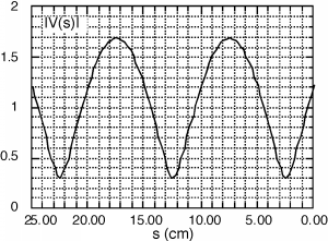
Figure \(\PageIndex{1}\): A standing wave pattern
Since , we can plot on the Smith Chart, as shown below in Figure \(\PageIndex{2}\). We do this by setting the compass at a radius of 0.7 and drawing a circle! Now, is somewhere on this circle. We just do not know where yet! There is more information to be gleaned from the VSWR plot, however.

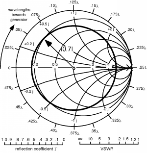
Figure \(\PageIndex{2}\): The VSWR circle
Firstly, we note that the plot has a periodicity of about 10 cm. This means that λ the wavelength of the signal on the line is 20 cm. Why? According to Equation 6.5.12, goes as and and , thus goes as . Thus each \(\frac{\lambda}{2}\), we are back to where we started.
Secondly, we note that there is a voltage minima at about 2.5 cm away from the load. Where on Figure \(\PageIndex{2}\) would we expect to find a voltage minima? It would be where has a phase angle of or point "A" shown in Figure \(\PageIndex{3}\). The voltage minima is always where the VSWR circle passes through the real axis on the left hand side. (Conversely a voltage maxima is where the circle goes through the real axis on the right hand side.) We don't really care about at a voltage minima, what we want is , the normalized load impedance. This should be easy! If we start at "A" and go towards the load we should end up at the point corresponding to . The arrow on the mini-Smith Chart says "Wavelengths towards generator" If we start at A, and want to go towards the load, we had better go around the opposite direction from the arrow. (Actually, as you can see on a real Smith Chart, there are arrows pointing in both directions, and they are appropriately marked for your convenience.)

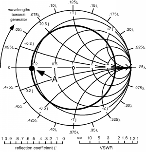
Figure \(\PageIndex{3}\): Location of a \(V_{\text{min}}\)
So we start at "A" go in a counterclockwise direction, and mark a new point "B" which represents our , which appears to be about or so, as in Figure \(\PageIndex{4}\). Thus, the load in this case (assuming a \(50 \text{-}\Omega\) line impedance) is a resistor, again by co-incidence of about \(50 \ \Omega\), in series with a capacitor with a negative reactance of about \(47.5 \ \Omega\). Note that we could have started at the minima at 12.5 cm or even 22.5 cm, and then have rotated or towards the load. Since \(\frac{\lambda}{2} = 0.5 \lambda\) means one complete rotation around the Smith Chart, we would have ended up at the same spot, with the same that we already have! We could also have started at a maxima, at say 7.5 cm, marked our starting point on the right hand side of the Smith chart, and then we would go counterclockwise and again, we'd end up at "B".

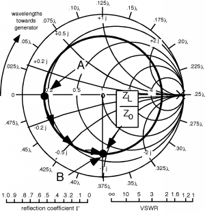
Figure \(\PageIndex{4}\): Moving from \(V_{\text{min}}\) to the load
Now, here in Figure \(\PageIndex{5}\) is another example. In this case the , which means and we get a circle as shown in Figure \(\PageIndex{6}\). The wavelength . The first minima is thus a distance of from the load. So we again start at the minima, "A" and now rotate as distance towards the load.

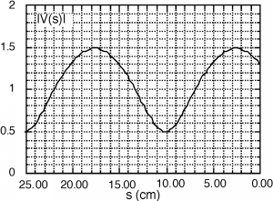
Figure \(\PageIndex{5}\): Another standing wave pattern

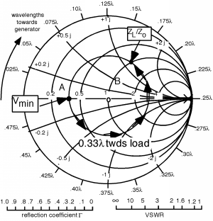
Figure \(\PageIndex{6}\): The VSWR circle