Engineering LibreTexts

6.14: Introduction to Parallel Matching

  • Page ID
    88586
  • \( \newcommand{\vecs}[1]{\overset { \scriptstyle \rightharpoonup} {\mathbf{#1}} } \) \( \newcommand{\vecd}[1]{\overset{-\!-\!\rightharpoonup}{\vphantom{a}\smash {#1}}} \)\(\newcommand{\id}{\mathrm{id}}\) \( \newcommand{\Span}{\mathrm{span}}\) \( \newcommand{\kernel}{\mathrm{null}\,}\) \( \newcommand{\range}{\mathrm{range}\,}\) \( \newcommand{\RealPart}{\mathrm{Re}}\) \( \newcommand{\ImaginaryPart}{\mathrm{Im}}\) \( \newcommand{\Argument}{\mathrm{Arg}}\) \( \newcommand{\norm}[1]{\| #1 \|}\) \( \newcommand{\inner}[2]{\langle #1, #2 \rangle}\) \( \newcommand{\Span}{\mathrm{span}}\) \(\newcommand{\id}{\mathrm{id}}\) \( \newcommand{\Span}{\mathrm{span}}\) \( \newcommand{\kernel}{\mathrm{null}\,}\) \( \newcommand{\range}{\mathrm{range}\,}\) \( \newcommand{\RealPart}{\mathrm{Re}}\) \( \newcommand{\ImaginaryPart}{\mathrm{Im}}\) \( \newcommand{\Argument}{\mathrm{Arg}}\) \( \newcommand{\norm}[1]{\| #1 \|}\) \( \newcommand{\inner}[2]{\langle #1, #2 \rangle}\) \( \newcommand{\Span}{\mathrm{span}}\)\(\newcommand{\AA}{\unicode[.8,0]{x212B}}\)

    Let's start with the load. With the same \(25 \ \Omega\) resistor for the load, and plot its admittance Y L Y 0 =2 Y L Y 0 2 . If we start moving away from the load towards the generator, in about 0.10λ 0.10 λ we again run into the circle which represents Ys Y 0 =1 Y s Y 0 1 . This is such an important circle is has gained its own name, and it is frequently called the matching circle shown in Figure \(\PageIndex{1}\).

    Mini Smith Chart with a VSWR circle of diameter 1 centered on the center of the Smith Chart has the chart circle corresponding to the real value of 1 marked as the "matching circle." The VSWR circle intersects the matching circle at point C above the horizontal axis and at point B below the horizontal axis. Point A, which corresponds to Y_L/Y_0, is the rightmost point of the VSWR circle, where it intersects the horizontal axis.

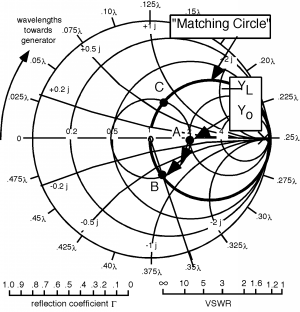
    Figure \(\PageIndex{1}\): Getting to the Matching Circle

    Note that to find out how far we had to move, we had to start at relative position 0.25λ 0.25 λ as our zero, or reference location. Point \(B\) seems to be at about 0.35λ 0.35 λ on the scale, and since we started at 0.25λ 0.25 λ , the distance is 0.350.25=0.10 0.35 0.25 0.10 . At point \(B\), Y s Y 0 =-1.0+0.7i Y s Y 0 -1.00.7 . Thus, if we add a susceptance iB B with a value of \(i 0.014 \ \Omega^{-1}\), we would again match the line. Positive susceptance comes from a capacitor as well, and so Figure \(\PageIndex{2}\) shows how we match.

    The right end of a transmission line contains a capacitor of susceptance j0.014 Siemens and a 25-Ohm resistor, connected in parallel by a line of length 0.10 lambda and impedance Z_0 of 50 Ohms. The input impedance to the parallel connection is equal to Z_0.

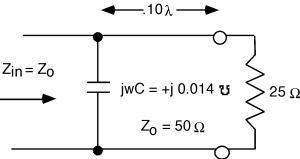
    Figure \(\PageIndex{2}\): Matching with a shunt capacitor

    Note that we are not required to go to point \(B\). Any point on the matching circle that we can get to is fair game. Another such point is \(C\) in Figure \(\PageIndex{1}\). This is at a distance of about 0.40λ 0.40 λ from the load. At \(C\), Y s Y 0 =1.0+0.7i Y s Y 0 1.00.7 and so we would put in an inductor, with a susceptance 1iωL=(i0.014Ω-1) 1 ω L 0.014 Ω -1  as in Figure \(\PageIndex{3}\).

    The right end of a transmission line contains an inductor of susceptance -j0.014 Siemens and a 25-Ohm resistor, connected in parallel by a line of length 0.40 lambda and impedance Z_0 of 50 Ohms. The input impedance to the parallel connection is equal to Z_0.

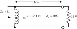
    Figure \(\PageIndex{3}\): Matching with a shunt inductor


    This page titled 6.14: Introduction to Parallel Matching is shared under a CC BY 1.0 license and was authored, remixed, and/or curated by Bill Wilson via source content that was edited to the style and standards of the LibreTexts platform; a detailed edit history is available upon request.

    • Was this article helpful?