6.15: Single Stub Matching
- Page ID
- 88587

\( \newcommand{\vecs}[1]{\overset { \scriptstyle \rightharpoonup} {\mathbf{#1}} } \)
\( \newcommand{\vecd}[1]{\overset{-\!-\!\rightharpoonup}{\vphantom{a}\smash {#1}}} \)
\( \newcommand{\dsum}{\displaystyle\sum\limits} \)
\( \newcommand{\dint}{\displaystyle\int\limits} \)
\( \newcommand{\dlim}{\displaystyle\lim\limits} \)
\( \newcommand{\id}{\mathrm{id}}\) \( \newcommand{\Span}{\mathrm{span}}\)
( \newcommand{\kernel}{\mathrm{null}\,}\) \( \newcommand{\range}{\mathrm{range}\,}\)
\( \newcommand{\RealPart}{\mathrm{Re}}\) \( \newcommand{\ImaginaryPart}{\mathrm{Im}}\)
\( \newcommand{\Argument}{\mathrm{Arg}}\) \( \newcommand{\norm}[1]{\| #1 \|}\)
\( \newcommand{\inner}[2]{\langle #1, #2 \rangle}\)
\( \newcommand{\Span}{\mathrm{span}}\)
\( \newcommand{\id}{\mathrm{id}}\)
\( \newcommand{\Span}{\mathrm{span}}\)
\( \newcommand{\kernel}{\mathrm{null}\,}\)
\( \newcommand{\range}{\mathrm{range}\,}\)
\( \newcommand{\RealPart}{\mathrm{Re}}\)
\( \newcommand{\ImaginaryPart}{\mathrm{Im}}\)
\( \newcommand{\Argument}{\mathrm{Arg}}\)
\( \newcommand{\norm}[1]{\| #1 \|}\)
\( \newcommand{\inner}[2]{\langle #1, #2 \rangle}\)
\( \newcommand{\Span}{\mathrm{span}}\) \( \newcommand{\AA}{\unicode[.8,0]{x212B}}\)
\( \newcommand{\vectorA}[1]{\vec{#1}} % arrow\)
\( \newcommand{\vectorAt}[1]{\vec{\text{#1}}} % arrow\)
\( \newcommand{\vectorB}[1]{\overset { \scriptstyle \rightharpoonup} {\mathbf{#1}} } \)
\( \newcommand{\vectorC}[1]{\textbf{#1}} \)
\( \newcommand{\vectorD}[1]{\overrightarrow{#1}} \)
\( \newcommand{\vectorDt}[1]{\overrightarrow{\text{#1}}} \)
\( \newcommand{\vectE}[1]{\overset{-\!-\!\rightharpoonup}{\vphantom{a}\smash{\mathbf {#1}}}} \)
\( \newcommand{\vecs}[1]{\overset { \scriptstyle \rightharpoonup} {\mathbf{#1}} } \)
\(\newcommand{\longvect}{\overrightarrow}\)
\( \newcommand{\vecd}[1]{\overset{-\!-\!\rightharpoonup}{\vphantom{a}\smash {#1}}} \)
\(\newcommand{\avec}{\mathbf a}\) \(\newcommand{\bvec}{\mathbf b}\) \(\newcommand{\cvec}{\mathbf c}\) \(\newcommand{\dvec}{\mathbf d}\) \(\newcommand{\dtil}{\widetilde{\mathbf d}}\) \(\newcommand{\evec}{\mathbf e}\) \(\newcommand{\fvec}{\mathbf f}\) \(\newcommand{\nvec}{\mathbf n}\) \(\newcommand{\pvec}{\mathbf p}\) \(\newcommand{\qvec}{\mathbf q}\) \(\newcommand{\svec}{\mathbf s}\) \(\newcommand{\tvec}{\mathbf t}\) \(\newcommand{\uvec}{\mathbf u}\) \(\newcommand{\vvec}{\mathbf v}\) \(\newcommand{\wvec}{\mathbf w}\) \(\newcommand{\xvec}{\mathbf x}\) \(\newcommand{\yvec}{\mathbf y}\) \(\newcommand{\zvec}{\mathbf z}\) \(\newcommand{\rvec}{\mathbf r}\) \(\newcommand{\mvec}{\mathbf m}\) \(\newcommand{\zerovec}{\mathbf 0}\) \(\newcommand{\onevec}{\mathbf 1}\) \(\newcommand{\real}{\mathbb R}\) \(\newcommand{\twovec}[2]{\left[\begin{array}{r}#1 \\ #2 \end{array}\right]}\) \(\newcommand{\ctwovec}[2]{\left[\begin{array}{c}#1 \\ #2 \end{array}\right]}\) \(\newcommand{\threevec}[3]{\left[\begin{array}{r}#1 \\ #2 \\ #3 \end{array}\right]}\) \(\newcommand{\cthreevec}[3]{\left[\begin{array}{c}#1 \\ #2 \\ #3 \end{array}\right]}\) \(\newcommand{\fourvec}[4]{\left[\begin{array}{r}#1 \\ #2 \\ #3 \\ #4 \end{array}\right]}\) \(\newcommand{\cfourvec}[4]{\left[\begin{array}{c}#1 \\ #2 \\ #3 \\ #4 \end{array}\right]}\) \(\newcommand{\fivevec}[5]{\left[\begin{array}{r}#1 \\ #2 \\ #3 \\ #4 \\ #5 \\ \end{array}\right]}\) \(\newcommand{\cfivevec}[5]{\left[\begin{array}{c}#1 \\ #2 \\ #3 \\ #4 \\ #5 \\ \end{array}\right]}\) \(\newcommand{\mattwo}[4]{\left[\begin{array}{rr}#1 \amp #2 \\ #3 \amp #4 \\ \end{array}\right]}\) \(\newcommand{\laspan}[1]{\text{Span}\{#1\}}\) \(\newcommand{\bcal}{\cal B}\) \(\newcommand{\ccal}{\cal C}\) \(\newcommand{\scal}{\cal S}\) \(\newcommand{\wcal}{\cal W}\) \(\newcommand{\ecal}{\cal E}\) \(\newcommand{\coords}[2]{\left\{#1\right\}_{#2}}\) \(\newcommand{\gray}[1]{\color{gray}{#1}}\) \(\newcommand{\lgray}[1]{\color{lightgray}{#1}}\) \(\newcommand{\rank}{\operatorname{rank}}\) \(\newcommand{\row}{\text{Row}}\) \(\newcommand{\col}{\text{Col}}\) \(\renewcommand{\row}{\text{Row}}\) \(\newcommand{\nul}{\text{Nul}}\) \(\newcommand{\var}{\text{Var}}\) \(\newcommand{\corr}{\text{corr}}\) \(\newcommand{\len}[1]{\left|#1\right|}\) \(\newcommand{\bbar}{\overline{\bvec}}\) \(\newcommand{\bhat}{\widehat{\bvec}}\) \(\newcommand{\bperp}{\bvec^\perp}\) \(\newcommand{\xhat}{\widehat{\xvec}}\) \(\newcommand{\vhat}{\widehat{\vvec}}\) \(\newcommand{\uhat}{\widehat{\uvec}}\) \(\newcommand{\what}{\widehat{\wvec}}\) \(\newcommand{\Sighat}{\widehat{\Sigma}}\) \(\newcommand{\lt}{<}\) \(\newcommand{\gt}{>}\) \(\newcommand{\amp}{&}\) \(\definecolor{fillinmathshade}{gray}{0.9}\)Often, there are reasons why using a discrete inductor or capacitor for matching is not such a good idea. At the high frequencies where matching is important, losses in both L or C mean that you don't get a good match, and most of the time (except for some air-dielectric adjustable capacitors) it is hard to get just the value you want.
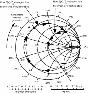
There is another approach, though. A shorted or open transmission line, when viewed at its input, looks like a pure reactance or pure susceptance. With a short as a load, the reflection coefficient has unity magnitude and so we move around the very outside of the Smith Chart as the length of the line increases or decreases, and is purely imaginary, in Figure \(\PageIndex{1}\). When we did the bilinear transformation from the plane to the plane, the imaginary axis transformed into the circle of diameter 2, which ended up being the outside circle which defined the Smith Chart.
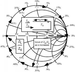
Figure \(\PageIndex{1}\): Input Impedance of a Shorted Line
Another way to see this is to go back to Equation 6.4.3. There we found:
With this reduces to
which, of course, for various values of , can take on any value from to . We don't have to go to Radio Shack© and buy a bunch of different inductor and capacitors. We can just get some transmission line and short it at various places!
Thus, instead of a discrete component, we can use a section of shorted (or open) transmission line instead, as shown in Figure \(\PageIndex{2}\). These matching lines are called matching stubs. One of the major advantages here is that with a line which has an adjustable short on the end of it, we can get any reactance we need, simply by adjusting the length of the stub. How this all works will become obvious after we take a look at an example.
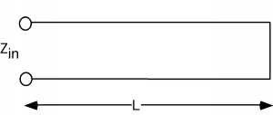
Figure \(\PageIndex{2}\): A shortened stub
Let's do one. In Figure \(\PageIndex{3}\) we can see that, , so we mark a point \(A\) on the Smith Chart. Since we will want to put the tuning or matching stub in shunt across the line, the first thing we will do is convert into a normalized admittance by going around the Smith Chart to point \(B\), where , as shown in Figure \(\PageIndex{4}\). Now we rotate around on the constant radius, circle until we hit the matching circle at point \(C\). This is shown in Figure \(\PageIndex{5}\). At \(C\), . Using a "real" Smith Chart, I get that the distance of rotation is about . Remember, all the way around is , so you can very often "eyeball" about how far you have to go, and doing so is a good check on making a stupid math error. If the distance doesn't look right on the Smith Chart, you probably made a mistake!
Figure \(\PageIndex{3}\): Another load
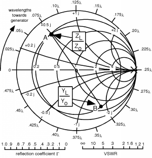
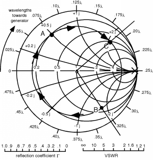
Figure \(\PageIndex{5}\): Moving to the matching circle
OK, at this point, the real part of the admittance is unity, so all we have to do is add a stub to cancel out the imaginary part. As mentioned above, the stubs often come with adjustable "sliding shorts" so we can make them whatever length we want as shown in Figure \(\PageIndex{6}\).
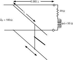
Figure \(\PageIndex{6}\): Matching with a shortened stub
Our task now, is to decide how much to push or pull on the sliding handle on the stub, to get the reactance we want. The hint on what we should do is in Figure \(\PageIndex{1}\). The end of the stub is a short circuit. What is the admittance of a short circuit? Answer: , ! Where is this on the Smith Chart? Answer: on the outside, on the right hand side on the real axis. Now, if we start at a short, and start to make the line longer than , what happens to ? It moves around on the outside of the Smith Chart. What we need to do is move away from the short until we get and we will know how long the shorted tuning stub should be Figure \(\PageIndex{7}\). In going from \(A\) to \(B\) we traverse a distance of about and so that is where we should set the position of the sliding short on the stub Figure \(\PageIndex{8}\).
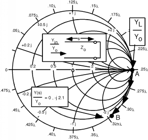
Figure \(\PageIndex{7}\): Finding the stub length
Figure \(\PageIndex{8}\): The matched line
We sometimes think of the action of the tuning stub as allowing us to move in along the to get to the center of the Smith Chart, or to a match, as shown in Figure \(\PageIndex{9}\). We are not in this case, physically moving down the line. Rather, we are moving along a contour of constant real part because all the stub can do is change the imaginary part of the admittance; it can do nothing to the real part!