
6.16: Double Stub Matching
- Page ID
- 88588

\( \newcommand{\vecs}[1]{\overset { \scriptstyle \rightharpoonup} {\mathbf{#1}} } \)
\( \newcommand{\vecd}[1]{\overset{-\!-\!\rightharpoonup}{\vphantom{a}\smash {#1}}} \)
\( \newcommand{\id}{\mathrm{id}}\) \( \newcommand{\Span}{\mathrm{span}}\)
( \newcommand{\kernel}{\mathrm{null}\,}\) \( \newcommand{\range}{\mathrm{range}\,}\)
\( \newcommand{\RealPart}{\mathrm{Re}}\) \( \newcommand{\ImaginaryPart}{\mathrm{Im}}\)
\( \newcommand{\Argument}{\mathrm{Arg}}\) \( \newcommand{\norm}[1]{\| #1 \|}\)
\( \newcommand{\inner}[2]{\langle #1, #2 \rangle}\)
\( \newcommand{\Span}{\mathrm{span}}\)
\( \newcommand{\id}{\mathrm{id}}\)
\( \newcommand{\Span}{\mathrm{span}}\)
\( \newcommand{\kernel}{\mathrm{null}\,}\)
\( \newcommand{\range}{\mathrm{range}\,}\)
\( \newcommand{\RealPart}{\mathrm{Re}}\)
\( \newcommand{\ImaginaryPart}{\mathrm{Im}}\)
\( \newcommand{\Argument}{\mathrm{Arg}}\)
\( \newcommand{\norm}[1]{\| #1 \|}\)
\( \newcommand{\inner}[2]{\langle #1, #2 \rangle}\)
\( \newcommand{\Span}{\mathrm{span}}\) \( \newcommand{\AA}{\unicode[.8,0]{x212B}}\)
\( \newcommand{\vectorA}[1]{\vec{#1}} % arrow\)
\( \newcommand{\vectorAt}[1]{\vec{\text{#1}}} % arrow\)
\( \newcommand{\vectorB}[1]{\overset { \scriptstyle \rightharpoonup} {\mathbf{#1}} } \)
\( \newcommand{\vectorC}[1]{\textbf{#1}} \)
\( \newcommand{\vectorD}[1]{\overrightarrow{#1}} \)
\( \newcommand{\vectorDt}[1]{\overrightarrow{\text{#1}}} \)
\( \newcommand{\vectE}[1]{\overset{-\!-\!\rightharpoonup}{\vphantom{a}\smash{\mathbf {#1}}}} \)
\( \newcommand{\vecs}[1]{\overset { \scriptstyle \rightharpoonup} {\mathbf{#1}} } \)
\( \newcommand{\vecd}[1]{\overset{-\!-\!\rightharpoonup}{\vphantom{a}\smash {#1}}} \)
\(\newcommand{\avec}{\mathbf a}\) \(\newcommand{\bvec}{\mathbf b}\) \(\newcommand{\cvec}{\mathbf c}\) \(\newcommand{\dvec}{\mathbf d}\) \(\newcommand{\dtil}{\widetilde{\mathbf d}}\) \(\newcommand{\evec}{\mathbf e}\) \(\newcommand{\fvec}{\mathbf f}\) \(\newcommand{\nvec}{\mathbf n}\) \(\newcommand{\pvec}{\mathbf p}\) \(\newcommand{\qvec}{\mathbf q}\) \(\newcommand{\svec}{\mathbf s}\) \(\newcommand{\tvec}{\mathbf t}\) \(\newcommand{\uvec}{\mathbf u}\) \(\newcommand{\vvec}{\mathbf v}\) \(\newcommand{\wvec}{\mathbf w}\) \(\newcommand{\xvec}{\mathbf x}\) \(\newcommand{\yvec}{\mathbf y}\) \(\newcommand{\zvec}{\mathbf z}\) \(\newcommand{\rvec}{\mathbf r}\) \(\newcommand{\mvec}{\mathbf m}\) \(\newcommand{\zerovec}{\mathbf 0}\) \(\newcommand{\onevec}{\mathbf 1}\) \(\newcommand{\real}{\mathbb R}\) \(\newcommand{\twovec}[2]{\left[\begin{array}{r}#1 \\ #2 \end{array}\right]}\) \(\newcommand{\ctwovec}[2]{\left[\begin{array}{c}#1 \\ #2 \end{array}\right]}\) \(\newcommand{\threevec}[3]{\left[\begin{array}{r}#1 \\ #2 \\ #3 \end{array}\right]}\) \(\newcommand{\cthreevec}[3]{\left[\begin{array}{c}#1 \\ #2 \\ #3 \end{array}\right]}\) \(\newcommand{\fourvec}[4]{\left[\begin{array}{r}#1 \\ #2 \\ #3 \\ #4 \end{array}\right]}\) \(\newcommand{\cfourvec}[4]{\left[\begin{array}{c}#1 \\ #2 \\ #3 \\ #4 \end{array}\right]}\) \(\newcommand{\fivevec}[5]{\left[\begin{array}{r}#1 \\ #2 \\ #3 \\ #4 \\ #5 \\ \end{array}\right]}\) \(\newcommand{\cfivevec}[5]{\left[\begin{array}{c}#1 \\ #2 \\ #3 \\ #4 \\ #5 \\ \end{array}\right]}\) \(\newcommand{\mattwo}[4]{\left[\begin{array}{rr}#1 \amp #2 \\ #3 \amp #4 \\ \end{array}\right]}\) \(\newcommand{\laspan}[1]{\text{Span}\{#1\}}\) \(\newcommand{\bcal}{\cal B}\) \(\newcommand{\ccal}{\cal C}\) \(\newcommand{\scal}{\cal S}\) \(\newcommand{\wcal}{\cal W}\) \(\newcommand{\ecal}{\cal E}\) \(\newcommand{\coords}[2]{\left\{#1\right\}_{#2}}\) \(\newcommand{\gray}[1]{\color{gray}{#1}}\) \(\newcommand{\lgray}[1]{\color{lightgray}{#1}}\) \(\newcommand{\rank}{\operatorname{rank}}\) \(\newcommand{\row}{\text{Row}}\) \(\newcommand{\col}{\text{Col}}\) \(\renewcommand{\row}{\text{Row}}\) \(\newcommand{\nul}{\text{Nul}}\) \(\newcommand{\var}{\text{Var}}\) \(\newcommand{\corr}{\text{corr}}\) \(\newcommand{\len}[1]{\left|#1\right|}\) \(\newcommand{\bbar}{\overline{\bvec}}\) \(\newcommand{\bhat}{\widehat{\bvec}}\) \(\newcommand{\bperp}{\bvec^\perp}\) \(\newcommand{\xhat}{\widehat{\xvec}}\) \(\newcommand{\vhat}{\widehat{\vvec}}\) \(\newcommand{\uhat}{\widehat{\uvec}}\) \(\newcommand{\what}{\widehat{\wvec}}\) \(\newcommand{\Sighat}{\widehat{\Sigma}}\) \(\newcommand{\lt}{<}\) \(\newcommand{\gt}{>}\) \(\newcommand{\amp}{&}\) \(\definecolor{fillinmathshade}{gray}{0.9}\)There is one last technique we can look at, which is somewhat more flexible than the single stub matching which we just looked at. This is called double stub matching! Suppose we have the following situation, as depicted in Figure \(\PageIndex{1}\). There is a load of located at the end of the line, and then some arbitrary distance away () an adjustable stub. Another (arbitrary) from the first stub, there is a second one. Let's plot on the Smith Chart in Figure \(\PageIndex{2}\), and then, since the stubs are in shunt across the line, switch to admittance, and find . It is easy to see that .

Figure \(\PageIndex{1}\): Double stub matching problem

Figure \(\PageIndex{2}\): Changing the load to an admittance
The first thing we might as well do is move down to the first stub, and see what admittance we have there, as shown in Figure \(\PageIndex{3}\). We go from the load, to the first stub by rotating on a circle of constant radius (constant )since all we are doing is going from one place on the line to another. If we call the location on the line of the first stub \(A\), then we can see that .
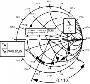
Figure \(\PageIndex{3}\): Moving from the load to the first stub
Now, what can the first stub accomplish? A shorted stub can create any imaginary admittance we want, but can not change the real part of the admittance. Thus, by adjusting the first stub, we can move around on a circle of constant real part , and have any imaginary part we want. This is shown schematically below in Figure \(\PageIndex{4}\).
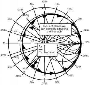
Figure \(\PageIndex{4}\): Possible effects of the first stub
Now, where do we want to go? Well, we would like to end up someplace so that, after we have moved from \(A\) to \(B\) on the line (gone from the first stub to the second), we are on the matching circle. If this were so, then, since we are on the matching circle, we could use the second stub to match the whole line and we would be done.
This is tricky now, so you have to pay attention and think. If I want to find a place which, when moved from \(A\) to \(B\), ends up on the matching circle, then what I should do is take the matching circle and move it from \(B\) to \(A\). That is, if I rotate the matching circle around towards the load, then any place on that rotated matching circle is guaranteed to end up on the real matching circle, when we go back towards the generator.
OK, so here's what we do. First, we rotate the matching circle 0.175 around towards the load (go counterclockwise), as in Figure \(\PageIndex{5}\). Now what we have to do is somehow get from without stub to someplace on the rotated matching circle. The only way we can do this is to change the imaginary part of with the stub. Suppose we move as shown in Figure \(\PageIndex{6}\). In going from without stub to with stub we have changed the imaginary part from to , thus we have added to the imaginary part of . Thus using our standard method for finding the length of the first stub, we start at , (the short at the end of the stub) and go around the outside of the Smith Chart until we find . To get from one place to the next we went and so the length of the first stub, should be . Now we are at with stub. The next thing we have to do is to rotate another towards the generator so that we can get to stub B. As we do this rotation, we again stay on a circle of constant radius, because now we are moving down the transmission line not adding reactance by using a stub! This rotation is guaranteed to end us up on the matching circle because every point on the rotated circle (the one we start from) is exactly towards the load from the matching circle. As shown in Figure \(\PageIndex{8}\), we are now at the point without stub . Thus we need to adjust the length of the second stub to give us of reactance, so we can move (along a circle of constant real part = 1.0) into the center of the Smith Chart in Figure \(\PageIndex{9}\). We have to find the length for the second stub, but that is now easy! (Figure \(\PageIndex{10}\))

Figure \(\PageIndex{5}\): Rotating the matching circle

Figure \(\PageIndex{6}\): Moving to rotated matching circle

Figure \(\PageIndex{7}\): Finding length of the first stub
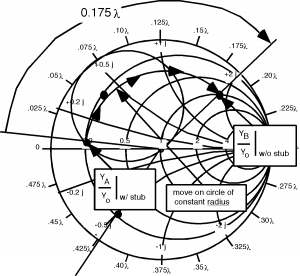
Figure \(\PageIndex{8}\): Moving down the second stub

Figure \(\PageIndex{9}\): Making the match

Figure \(\PageIndex{10}\): Finding the length of the second stub
Thus, by doing double stub matching, we are able, by adding the additional degree of freedom of two adjustable stubs, not to have to specify exactly where the stubs have to be placed, so they can be in the line before the matching is attempted. Figure \(\PageIndex{11}\) below shows the whole sequence of changes that we made. See if you can begin at "Start" and go through the numbers and get from to the matching point at the center of the Smith Chart. Remember, when we move from one place to another on the line, we must stay on a circle of constant radius. When we change reactance by adjusting a stub, we must move along circles of constant real part. If you do that, it's easy!

Figure \(\PageIndex{11}\): Double stub matching all put together!
There's just one little problem. What if without stub had ended up as shown in Figure \(\PageIndex{12}\). We are on the circle. No matter how hard I try, and no matter where I set , all I can do is spin around on the little circle as shown, and I will never end up on the rotated matching circle, and I won't be able to make a match! Well, if I add a third stub...I'll let you work it out!

Figure \(\PageIndex{12}\): A situation that doesn't work