3.3: Polar Representations of Scattering Parameters

Last updated
Save as PDF

Page ID: 41100

\( \newcommand{\vecs}[1]{\overset { \scriptstyle \rightharpoonup} {\mathbf{#1}} } \) \( \newcommand{\vecd}[1]{\overset{-\!-\!\rightharpoonup}{\vphantom{a}\smash {#1}}} \)\(\newcommand{\id}{\mathrm{id}}\) \( \newcommand{\Span}{\mathrm{span}}\) \( \newcommand{\kernel}{\mathrm{null}\,}\) \( \newcommand{\range}{\mathrm{range}\,}\) \( \newcommand{\RealPart}{\mathrm{Re}}\) \( \newcommand{\ImaginaryPart}{\mathrm{Im}}\) \( \newcommand{\Argument}{\mathrm{Arg}}\) \( \newcommand{\norm}[1]{\| #1 \|}\) \( \newcommand{\inner}[2]{\langle #1, #2 \rangle}\) \( \newcommand{\Span}{\mathrm{span}}\) \(\newcommand{\id}{\mathrm{id}}\) \( \newcommand{\Span}{\mathrm{span}}\) \( \newcommand{\kernel}{\mathrm{null}\,}\) \( \newcommand{\range}{\mathrm{range}\,}\) \( \newcommand{\RealPart}{\mathrm{Re}}\) \( \newcommand{\ImaginaryPart}{\mathrm{Im}}\) \( \newcommand{\Argument}{\mathrm{Arg}}\) \( \newcommand{\norm}[1]{\| #1 \|}\) \( \newcommand{\inner}[2]{\langle #1, #2 \rangle}\) \( \newcommand{\Span}{\mathrm{span}}\)\(\newcommand{\AA}{\unicode[.8,0]{x212B}}\)

Scattering parameters are most naturally represented in polar form with the square of the magnitude relating to power flow. In this section a greater rationale for representing \(\text{S}\) parameters on a polar plot is presented and this serves as the basis for a more complicated representation of \(\text{S}\) parameters on a Smith chart to be described in the next section.

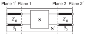
Figure \(\PageIndex{1}\): A two-port with scattering parameter matrix \(\mathbf{S}\) augmented by lines at each port with the line at Port \(n\) having the reference characteristic impedance at that port, i.e. \(Z_{0n}\) and with electrical length (in radians) of \(\theta_{n}\). The scattering parameter matrix of the augmented two-port is \(\mathbf{S}'\).

3.3.1 Shift of Reference Planes as a S Parameter Rotation

A polar plot is a natural way to present \(S\) parameters graphically. In general \(S\) parameters are referenced to different characteristic impedances \(Z_{0n}\) at each port. Adding additional lengths of the lines at each port rotates the \(S\) parameters. Consider the two-port in Figure \(\PageIndex{1}\). Here the original two-port with scattering parameter matrix \(\mathbf{S}\) is augmented by lines at each port with each having a characteristic impedance equal to the reference impedance. The \(S\) parameter matrix of the augmented two-port, \(\mathbf{S}'\), are the same as the original \(S\) parameter matrix but phase-shifted. That is

\[\label{eq:1}\mathbf{S}'=\left[\begin{array}{cc}{S_{11}'}&{S_{12}'}\\{S_{21}'}&{S_{22}'}\end{array}\right]=\left[\begin{array}{cc}{S_{11}\text{e}^{-\jmath 2\theta 1}}&{S_{12}\text{e}^{-\jmath (\theta 1+\theta 2)}} \\ {S_{21}\text{e}^{-\jmath (\theta 1+\theta 2)}}&{S_{22}\text{e}^{-\jmath 2\theta 2}}\end{array}\right] \]

The shift in reference planes simply rotates the \(S\) parameters. This is one of the main reasons why \(S\) parameters are commonly plotted on a polar plot.

3.3.2 Polar Plot of Reflection Coefficient

The polar plot of reflection coefficient is simply the polar plot of a complex number. Figure \(\PageIndex{2}\) is used in plotting reflection coefficients and is a polar plot that has a radius of one. So a reflection coefficient with a magnitude of one is on the unit circle. The center of the polar plot is zero so the reflection coefficient of a matched load, which is zero, is plotted at the center of the circle. Plotting a reflection coefficient on the polar plot enables convenient interpretation of the properties of a reflection. The graph has additional notation that enables easy plotting of an \(S\) parameter on the graph. Conversely, the magnitude and phase of an \(S\) parameter can be easily read from the graph. The horizontal label going from \(0\) to \(1\) is used in determining magnitude. The notation arranged on the outer perimeter of the polar plot is used to read off angle information. Notice the additional notation “ANGLE OF REFLECTION COEFFICIENT IN DEGREES” and the scale relates to the actual angle of the polar plot. Verify that the \(90^{\circ}\) point is just where one would expect it to be.

Figure \(\PageIndex{3}\) annotates the polar plot of reflection coefficient with real and imaginary axes and shows the location of the short circuit and open circuit points. Note that the reflection coefficient of an inductive impedance is in the top half of the polar plot while the reflection coefficient of a capacitive impedance is in the bottom half of the polar plot.

The nomograph shown in Figure \(\PageIndex{4}\) aids in interpretation of polar reflection coefficient plots. The nomograph relates the reflection coefficient (RFL. COEFFICIENT), \(\rho\) (\(\rho\) was originally used instead of \(\Gamma\) and is still used with the Smith chart); the return loss (RTN. LOSS) (in decibels); and the standing wave ratio (SWR); and the standing wave ratio (in decibels) as \(20 \log(\text{SWR})\). When printed together with the reflection coefficient polar plot (Figures \(\PageIndex{2}\) and \(\PageIndex{4}\) combined) the nomograph is scaled properly, but

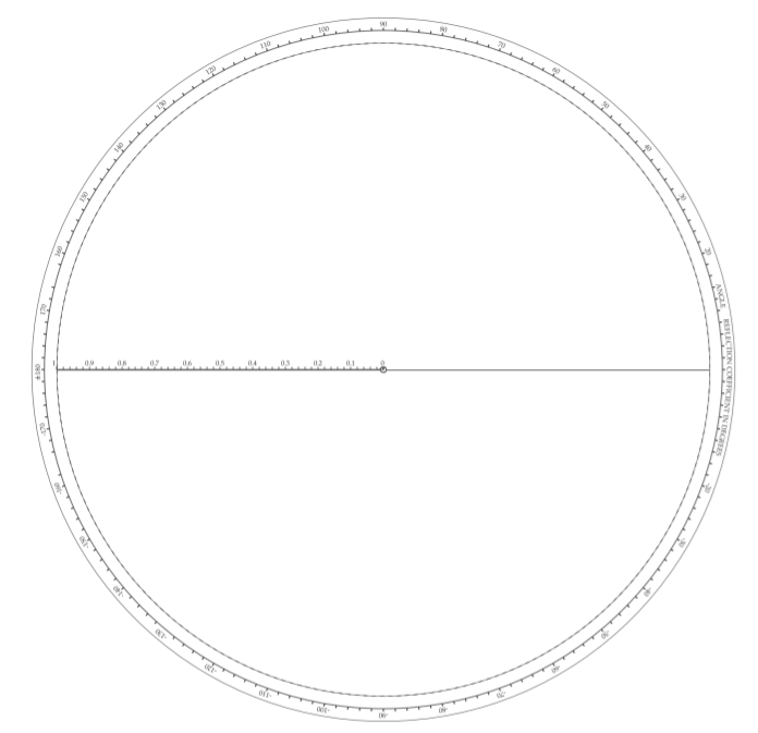
Figure \(\PageIndex{2}\): Polar chart for plotting reflection coefficient and transmission coefficient.

it is expanded here so that it can be read more easily. So with the aid of a compass with one point on the zero point of the polar plot and the other at the reflection coefficient (as plotted on the polar plot), the magnitude of the reflection coefficient is captured. The compass can then be brought down to the nomograph to read \(\rho\), the return loss, and VSWR directly.

3.3.3 Summary

This section introduced the plotting of reflection coefficients as a complex number on a polar plot. The use of angle and magnitude scales make it easy to plot a complex number in magnitude-angle form but it is also easy to plot or read-off the complex number in real-imaginary form. Nomographs also enable return loss and SWR to be developed without calculation. The

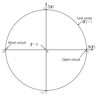
Figure \(\PageIndex{3}\): Annotated polar plot of reflection coefficient with real, \(\Re\), and imaginary, \(\Im\), axes. The short circuit \(\Gamma = −1\) and open circuit \(\Gamma = +1\) are indicated. The reflection coefficient is referenced to a reference impedance \(Z_{REF}\). Thus an impedance \(Z_{L}\) has the reflection coefficient \(\Gamma =(Z_{L} − Z_{\text{REF}})/(Z_{L} + Z_{\text{REF}})\)). An interesting observation is that the angle of \(\Gamma\) when \(Z_{L}\) is inductive, i.e. has a positive reactance, has a positive angle between \(0^{\circ}\) and \(180^{\circ}\) and so \(\Gamma\) is in the top half of the polar plot. Similarly the angle of \(\Gamma\) when \(Z_{L}\) is capacitive, i.e. has a negative reactance, has a negative angle between \(0^{\circ}\) and \(−180^{\circ}\) and so \(\Gamma\) is in the bottom half of the polar plot.

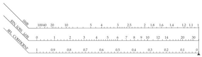
Figure \(\PageIndex{4}\): Nomograph relating the reflection coefficient (RFL. COEFFICIENT), \(\rho\); the return loss (RTN. LOSS) (in decibels); and the standing wave ratio (SWR).

transmission coefficient can be plotted on the same polar plot, i.e. Figure \(\PageIndex{2}\), as the polar plot is the representation of a complex number.