3.4: Smith Chart

The Smith chart is a powerful graphical tool used in the design of microwave circuits. Mastering the Smith chart is essential to entering the world of RF and microwave circuit design as all practitioners use this as if it is well understood by others. It takes effort to master but fundamentally it is quite simple combining a polar plot used for plotting \(S\) parameters directly, curves that enable normalized impedances and admittances to be plotted directly, and scales that enable electrical lengths in terms of wavelengths and degrees to be read off. The chart has many numbers printed in quite small font and with signs dropped as there is not room.

The Smith chart was invented by Phillip Smith and presented in close to its current form in 1937, see [7, 8, 9, 10]. Once nomographs and graphical calculators were common engineering tools mainly because of limited computing resources. Only a few have survived in electrical engineering usage, with Smith charts being overwhelmingly the most important.

This section first presents the impedance Smith chart and then the admittance Smith chart before introducing a combined Smith chart which is the form needed in design. The Smith chart presents a large amount of information in a confined space and interpretation, such as applying appropriate signs, is required to extract values. The Smith chart is a ‘backof-the-envelope’ tool that designers use to sketch out designs.

3.4.1 Impedance Smith Chart

The reflection coefficient, \(\Gamma\), is related to a load, \(Z_{L}\), by

\[\label{eq:1}\Gamma=\frac{Z_{L}-Z_{\text{REF}}}{Z_{L}+Z_{\text{REF}}} \]

where \(Z_{\text{REF}}\) is the system reference impedance. With normalized load impedance \(z_{l} = r +\jmath x = Z_{L}/Z_{\text{REF}}\), this becomes

\[\label{eq:2}\Gamma=\frac{r+\jmath x-1}{r+\jmath x+1} \]

Commonly in network design reactive elements are added either in shunt or in series to an existing network. If a reactive element is added in series then the input reactance, \(x\), is changed while the input resistance, \(r\), is held constant. So superimposing the loci of \(\Gamma\) (on the \(S\) parameter polar plot) with fixed values of \(r\), but varying values of \(x\) (\(x\) varying from \(−∞\) to \(∞\)), proves useful, as will be seen. Another loci of \(\Gamma\) with fixed values of \(x\) and varying values of \(r\) (\(r\) varying from \(0\) to \(∞\)) is also useful. The combination of the reflection/transmission polar plots, the nomographs, and the \(r\) and \(x\) loci is called the impedance Smith chart, see Figure \(\PageIndex{1}\). This is still a polar plot of reflection coefficient and the arcs and circles of constant and resistance enable easy conversion between reflection coefficient and impedance.

The full impedance Smith chart shown in Figure \(\PageIndex{1}\) is daunting so discussion will begin with the less dense form of the impedance Smith chart shown in Figure \(\PageIndex{2}\)(a) which is annotated in Figure \(\PageIndex{2}\)(b). Referring to Figure \(\PageIndex{2}\)(b), the unit circle corresponds to a reflection coefficient magnitude of one and hence a pure reactance. Note that there are lines of constant resistance and arcs of constant reactance. All points in the top half of the Smith chart have positive reactances and so all reflection coefficient points plotted in the top half of the Smith chart indicate inductive impedances. All points in the bottom half of the Smith chart have negative reactances and so all reflection coefficient points plotted in the bottom half of the Smith chart indicate capacitive impedances. The horizontal line across the middle of the Smith chart indicates pure resistance.

A point on the unit circle indicate that the resistance of the point is zero, while a reflection coefficient point inside the unit circle indicates a finite positive resistance.

One big difference between the less dense form of the impedance Smith chart, Figure \(\PageIndex{2}\)(a), and the full impedance Smith chart of Figure \(\PageIndex{1}\) is that the signs of the reactances are missing in the full impedance Smith chart. This is simply because there is not enough room and the user must add the appropriate sign when reading the chart. Thus it is essential that the user keep the annotations in Figure \(\PageIndex{2}\)(b) in mind. Yet another factor that makes it difficult to develop essential Smith chart skills.

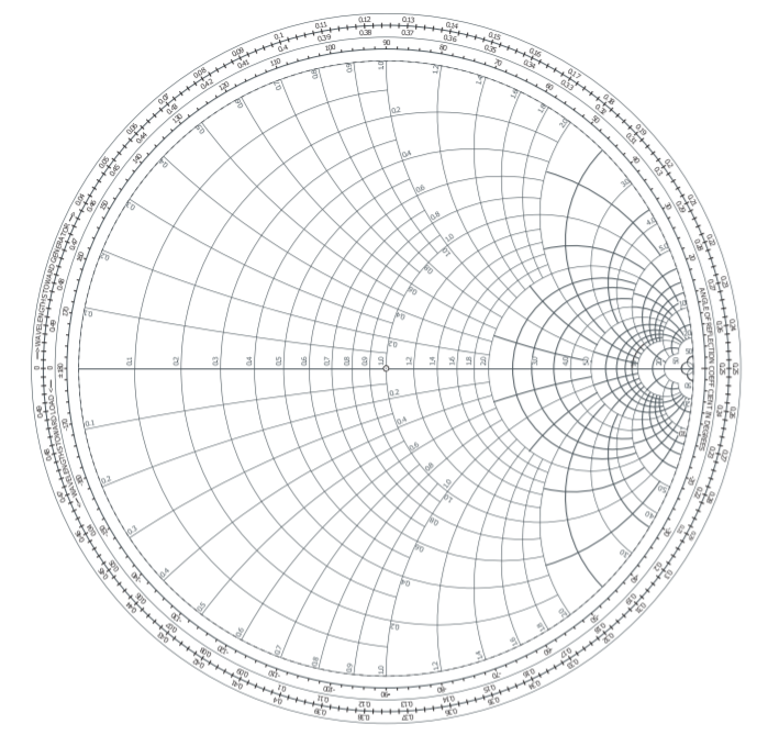
Figure \(\PageIndex{1}\): Impedance Smith chart. Also called a normalized Smith chart since resistances and reactances have been normalized to the system reference impedance \(Z_{\text{REF}}:\: z = Z/Z_{\text{REF}}\). A point plotted on the Smith chart represents a complex number \(A\). The magnitude of A is obtained by measuring the distance from the origin of the polar plot (the same as the origin of the Smith chart in the center of the unit circle) to point \(A\), say using a ruler, and comparing that to the measurement of the radius of the unit circle which corresponds to a complex number with a magnitude of 1. The angle in degrees of the complex number \(A\) is read from the innermost circular scale. The technique used is to draw a straight line from the origin through point \(A\) out to the circular scale.

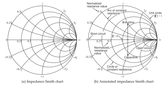
Figure \(\PageIndex{2}\): Normalized impedance Smithe charts.

Example \(\PageIndex{1}\): Impedance Plotting

Plot the normalized impedances \(z_{A} = 1 − 2\jmath\) and \(zB_{ }= 0.3+0.6\jmath\) on an impedance Smith chart.

Solution

The impedance \(z_{A} = 1 − 2\jmath\) is plotted as Point \(\mathsf{A}\) to the right. To plot this, first identify the circle of constant normalized resistance \(r = 1\), and then identify the arc of constant normalized reactance \(x = −2\). The intersection of the circle and arc locates \(z_{A}\) at point \(\mathsf{A}\). The reader is encouraged to do this with the full impedance Smith chart as shown in Figure \(\PageIndex{1}\). Recall that signs of reactances are missing on the full chart. As an exercise read off the reflection coefficient (the answer is \(0.5−\jmath .5=0.707\angle −45^{\circ}\)).

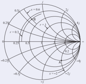
Figure \(\PageIndex{3}\)

The impedance \(z_{B} = 0.3 + 0.6\jmath\) is plotted as Point \(\mathsf{B}\) which is at the intersection of the circle \(r = 0.3\) and the arc \(x = +0.6\). Interpolation is required to identify the required circle and arc. The reader should do this with the full impedance Smith chart. As an exercise read off the reflection coefficient (the answer is \(−0.268 +\jmath 0.585 = 0.644\angle 115^{\circ}\)).

Example \(\PageIndex{2}\): Impedance Synthesis

Use a length of terminated transmission line to realize an impedance of \(Z_{\text{in}} = \jmath 140\:\Omega\).

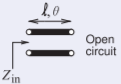
Figure \(\PageIndex{4}\)

Solution

The impedance to be synthesized is reactive so the termination must also be lossless. The simplest termination is either a short circuit or an open circuit. Both cases will be considered. Choose a transmission line with a characteristic impedance, \(Z_{0}\), of \(100\:\Omega\) so that the desired normalized input impedance is \(\jmath 140\:\Omega /Z_{0} = 1.4\jmath\), plotted as point \(\mathsf{B}\) in Figure \(\PageIndex{6}\).

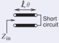
Figure \(\PageIndex{5}\)

First, the short-circuit case. In Figure \(\PageIndex{6}\), consider the path \(\mathsf{AB}\). The termination is a short circuit and the impedance of this load is Point \(\mathsf{A}\) with a reference length of \(\ell_{A} = 0\:\lambda\) (from the outermost circular scale). The corresponding reflection coefficient reference angle from the scale is \(\theta_{A} = 180^{\circ}\) (from the innermost circular scale labeled ‘WAVELENGTHS TOWARDS THE GENERATOR’ which is the same as ‘wavelengths away from the load’). As the line length increases, the input impedance of the terminated line follows the clockwise path to Point \(\mathsf{B}\) where the normalized input impedance is \(\jmath 1.4\). (To verify your understanding that the locus of the refection coefficient rotates in the clockwise direction, i.e. increasingly negative angle, as the line length increases see Section 2.3.3 of [11].) At Point \(\mathsf{B}\) the reference line length \(\ell_{B} = 0.1515\:\lambda\) and the corresponding reflection coefficient reference angle from the scale is \(\theta_{B} = 71.2^{\circ}\). The reflection coefficient angle and length in terms of wavelengths were read directly off the Smith chart and care needs to be taken that the right sign and correct scale are used. A good strategy is to correlate the scales with the easily remembered properties at the open-circuit and short-circuit points. Here the line length is

\[\label{eq:3}\ell=\ell_{B}-\ell_{A}=0.1515\lambda -0\lambda =0.1515\lambda \]

and the electrical length is half of the difference in the reflection coefficient angles,

\[\label{eq:4}\theta=\frac{1}{2}\left|\theta_{B}-\theta_{A}\right|=\frac{1}{2}\left|71.2^{\circ}-180^{\circ}\right|=54.4^{\circ} \]

corresponding to a length of \((54.4^{\circ}/360^{\circ})\lambda = 0.1511\lambda\) (the discrepancy with the previously determine line length of \(0.1515\lambda\) is small). This is as close as could be expected from using the scales. So the length of the stub with a short-circuit termination is \(0.1515\lambda\).

For the open-circuited stub, the path begins at the infinite impedance point \(\Gamma = +1\) and rotates clockwise to Point \(\mathsf{A}\) (this is a \(90^{\circ}\) or \(0.25\lambda\) rotation) before continuing on to Point \(\mathsf{B}\). For the open-circuited stub,

\[\label{eq:5}\ell=0.1515\lambda+0.25\lambda=0.4015\lambda \]

3.4.2 Admittance Smith Chart

The admittance Smith chart has loci for discrete constant susceptances ranging from \(−∞\) to \(∞\), and for discrete constant conductance ranging from \(0\) to \(∞\), see Figure \(\PageIndex{7}\). A less dense form is shown in Figure \(\PageIndex{8}\)(a). This chart looks like the flipped version of the impedance Smith chart but it is the same polar plot of a reflection coefficient so that the positions of the open and short circuit remain the same as do the capacitive and inductive halves of the Smith chart. In the full version of the admittance Smith chart, Figure \(\PageIndex{7}\), signs have been dropped as there is not room for them. Thus interpreting admittances from the chart requires that the user separately determine the signs of susceptances. The less dense version, Figure \(\PageIndex{8}\)(a), retains the signs making it easier to follow some of the discussions and examples. It is important that the user readily understand the annotations on the less dense form of the Smith chart, see Figure \(\PageIndex{8}\)(b).

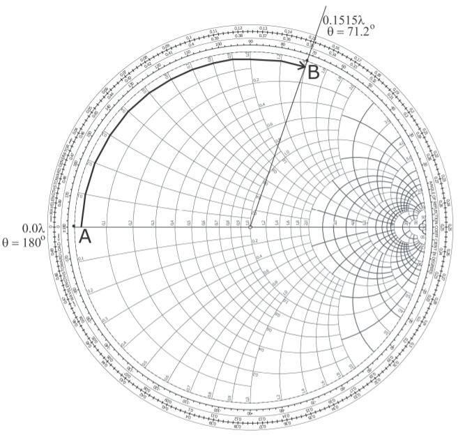
Figure \(\PageIndex{6}\): Design of a short-circuit stub with a normalized input impedance of \(\jmath 1.4\). The path \(\mathsf{AB}\) is actually on the unit circle but has been displaced here to avoid covering numbers. The electrical length in wavelengths has been read from the outermost circular scale, and the angle, \(\theta\), in degrees refers to the angle of the polar plot (and is twice the electrical length).

3.4.3 Combined Smith Chart

The combination of the reflection/transmission polar plots, nomographs, and the impedance and admittance Smith chart leads to the combined Smith chart (see Figure \(\PageIndex{9}\)). This color Smith chart is the preferred version for use in design and the separate impedance and admittance versions of the Smith chart are rarely used. The combined Smith charts is rich with information and care is required to identify the lines that correspond to admittances (specifically lines of constant normalized conductance and constant normalized susceptances), and the lines that correspond to impedances (constant normalized resistances and constant normalized

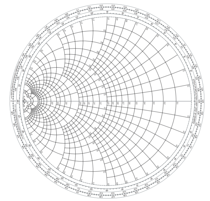
Figure \(\PageIndex{7}\): Admittance Smith chart.

reactances). The signs of the reactances and susceptible are missing and left to the user to add them depending on whether a reflection coefficient point is capacitive (in the lower half of the Smith chart and hence susceptances are positive and reactances are negative) or whether a point is inductive (in the upper half of the Smith chart and hence susceptances are negative and reactances are positive). A less dense version of the combined Smith chart, with the addition of signs, is shown in Figure \(\PageIndex{10}\)(a).

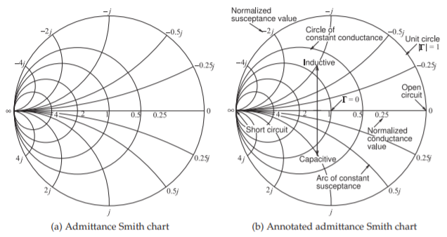
Figure \(\PageIndex{8}\): Normalized admittance Smith chart.

Example \(\PageIndex{3}\): Impedance to Admittance Conversion

Use a Smith chart to convert the impedance \(z = 1 − 2\jmath\) to an admittance.

Solution

The impedance \(z = 1−2\jmath\) is plotted as Point \(\mathsf{A}\) in Figure \(\PageIndex{10}\)(b). To read the admittance from the chart, the lines of constant conductance and constant susceptance must be interpolated from the arcs and circles provided. The interpolations are shown in the figure, indicating a conductance of \(0.2\) and a susceptance of \(0.4\jmath\). Thus

\[y=0.2+0.4\jmath\nonumber \]

(This agrees with the calculation: \(y = 1/z = 1/(1 − 2\jmath )=0.2+0.4\jmath\).)

Adding Reactance and Susceptance

A good amount of microwave design, such as designing a matching network for maximum power transfer, involves beginning with a load impedance plotted on a Smith chart and inserting series and shunt reactances, and transmission lines, to transform the impedance to another value. The preferred view of the design process is that of a reflection coefficient that gradually evolves from one value to another. That is, in the case of a series reactance, the effect is that of a reflection coefficient gradually changing as the reactances increase from zero to its actual value. The path traced out by the gradually evolving reflection coefficient value is called a locus. The loci of common circuit elements added to various loads are shown in Figure \(\PageIndex{11}\). For each locus the load is at the start of the arrow with the value of the element increasing from zero to its actual final value at the arrow head.

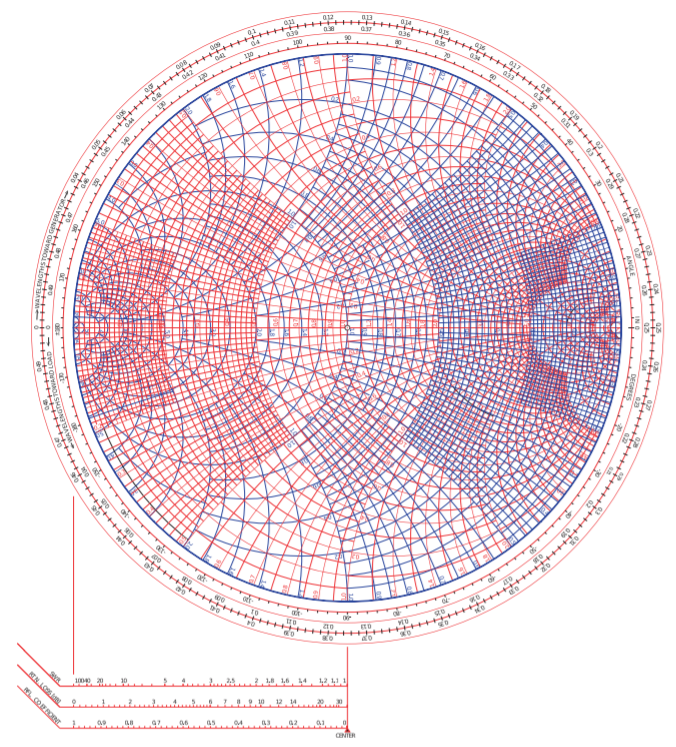
Figure \(\PageIndex{9}\): Normalized combined Smith chart combining impedance and admittance Smith charts.

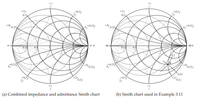
Figure \(\PageIndex{10}\): Combined impedance and admittance Smith chart.

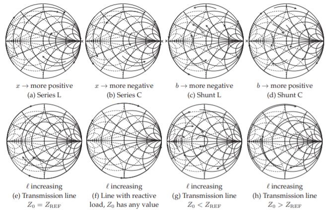
Figure \(\PageIndex{11}\): Reflection coefficient locus of a load augmented by elements as indicated. The original load is at the start of the arrowed arc. In (a) and (b) the locus is with respect to increasing \(|x|\) (normalized reactance magnitude), in (c) and (d) the locus is with respect to increasing \(|b|\) (normalized susceptance magnitude), and in (e)–(h) with respect to increasing length \(\ell\). In (e)– (h) the loci are parts of circles centered on the \(x = 0\) line. \(x\) indicates that the locus cannot cross infinity (open circuit for (a) and (b), short circuit for (c) and (d)).

3.4.4 Smith Chart Manipulations

Microwave design often proceeds by taking a known load and transforming it into another impedance, perhaps for maximum power transfer. Smith charts are used to show these manipulations. In design the manipulations required are not known up front and the Smith chart enables identification of those required. Except for particular situations, lossless elements such as reactances and transmission lines are used. The few situations where resistances are introduced include introducing stability in oscillators and amplifiers, and deliberately reduce signals levels. Most of the time introducing resistances unnecessarily increases noise and reduces signal levels thus reducing critical signal-to-noise ratios.

The circuit in Figure \(\PageIndex{12}\) will be used to illustrate the representation of manipulations on a Smith chart. The most common view is to consider that the Smith chart is a plot of the reflection coefficient at various stages in the circuit, i.e., \(\Gamma_{A},\: \Gamma_{B},\: \Gamma_{C},\: \Gamma_{D}\), and \(\Gamma_{\text{IN}}\). Additionally the load, \(Z_{L}\), is plotted and reactances, susceptances, or transmission lines transform the reflection coefficient from one stage to the next. Yet another concept is the idea that the effect of an element is regarded as gradually increasing from a negligible value up to the final actual value and in so doing tracing out a locus which ends in an arrow head. This is the approach nearly all RF and microwave engineers use. The manipulations corresponding to the circuit are illustrated in Figure \(\PageIndex{13}\). The individual steps are identified in Figure \(\PageIndex{14}\). The first few steps are confined to the top half of the Smith chart which is repeated on a larger scale in Figure \(\PageIndex{15}\) for the first three steps.

Step 1 \(\mathsf{L, a, b, c, d, e, f}\)
The first step is to plot the load \(Z_{L}\) on a Smith chart and this is the Point \(\mathsf{L}\) in Figures \(\PageIndex{13}\)–\(\PageIndex{15}\). The reference impedance \(Z_{\text{REF}}\) is chosen to be \(50\:\Omega\), the same as the characteristic impedance of the transmission line in the circuit. The Smith chart is now known as a \(50-\Omega\) Smith chart. This is a common choice because then the locus of reflection coefficient variation introduced by the line will be a circle centered at the origin of the Smith chart. To plot \(\mathsf{L}\) derive the normalized load impedance \(z_{L} = Z_{L}/Z_{\text{REF}} = 0.3 +\jmath 0.6\) (future numerical values are given in Figure \(\PageIndex{12}\)).

To plot \(z_{L}\) the normalized resistance circle for \(0.3\) and the normalized

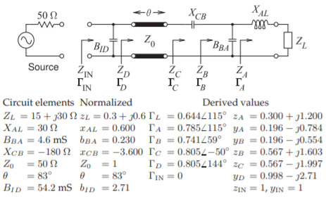
Figure \(\PageIndex{12}\): Circuit used in illustrating Smith chart manipulations. \(Z_{\text{REF}} = 50\:\Omega,\: Y_{\text{REF}} = 1/Z_{\text{REF}}= 20\text{ mS},\: z = Z/Z_{\text{REF}},\: y = Y/Y_{\text{REF}},\: Z_{\text{IN}} = Z_{\text{REF}} = 50\:\Omega\). In the circuit \(B\) indicates susceptance and \(X\) indicates reactance.

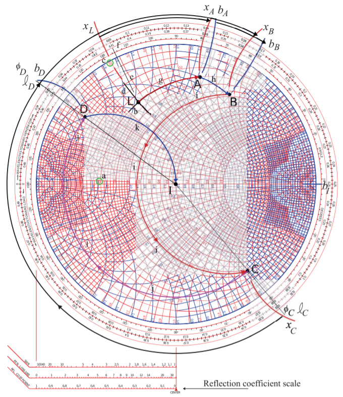
Figure \(\PageIndex{13}\): Smith chart manipulations corresponding to the circuit in Figure \(\PageIndex{12}\) with circuit elements added one at a time beginning with the load impedance at Point \(\mathsf{L}\).

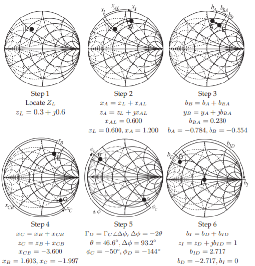
Figure \(\PageIndex{14}\): Steps in the Smith chart manipulations shown in Figures \(\PageIndex{13}\) and \(\PageIndex{15}\).

reactance arc for \(+0.3\) must be located. The resistance circle is identified from the scale on the horizontal axis of the Smith chart, see the circled value labeled ‘\(\mathsf{a}\)’. Locating the \(+0.3\) reactance arc is not as direct as the signs of reactance are missing on the Smith chart. Referring back to Figure \(\PageIndex{2}\) it is noted that an inductive impedance is in the top half of the Smith chart and so positive reactances are in the top half. Thus the \(+0.3\) reactance arc is in the top half of the Smith chart and the correct arc is identified by ‘\(\mathsf{c}\)’. From the curves identified by ‘\(\mathsf{a}\)’ and ‘\(\mathsf{c}\)’ the arcs ‘\(\mathsf{b}\)’ and ‘\(\mathsf{d}\)’ are drawn with the impedance \(z_{L}\), i.e. point \(\mathsf{L}\), at the intersection of the arcs.

It is instructive to determine \(\Gamma_{L}\), the reflection coefficient at \(\mathsf{L}\). On the Smith chart the reflection coefficient vector \(\Gamma_{L}\) is drawn from the origin to the point \(\mathsf{L}\). \(\Gamma_{L}\) is evaluated by separately determining its magnitude and angle. To determine the magnitude measure the length of the \(\Gamma_{L}|\) vector either using a ruler, a compass, or marking the edge of a piece of paper. Then this length can be compared against the reflection coefficient scale shown at the bottom of Figure \(\PageIndex{13}\) yielding \(|\Gamma_{L}| = 0.644\). The angle of \(\Gamma_{L}\) is read by extending the \(\Gamma_{L}\) vector out to the inner most circular scale on the Smith chart. This extension is labeled as e. The angle is read at point ‘\(\mathsf{f}\)’ as \(115^{\circ}\). Thus \(\Gamma_{L} = 0.644\angle 115^{\circ}\).

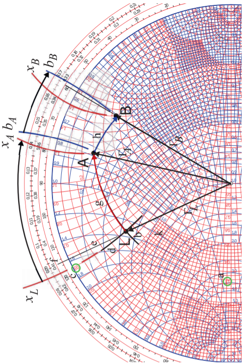
Figure \(\PageIndex{15}\): The first three steps in the Smith chart manipulations in Figure \(\PageIndex{13}\).

Step 2 Add the series reactance \(X_{AL}\), path \(\mathsf{L}\) to \(\mathsf{A, g}\)
In step 2 an inductor with reactance \(X_{AL}\) is in series with \(Z_{L}\) and the reflection coefficient transitions from point \(\mathsf{L}\) to point \(\mathsf{A}\). Now \(x_{L} = \Im\{z_{L}\} = 0.6\). To this \(x_{AL} = 0.6\) is added so that the normalized reactance at \(\mathsf{A}\) is \(x_{A} = x_{L} + x_{AL} = 0.6+0.6=1.2\). The locus of this operation is the arc, ‘\(\mathsf{g}\)’, extending from \(\mathsf{L}\) with gradually increasing series reactance until the full value \(x_{AL}\), at the arrowhead of the locus, is obtained. The procedure is to identify the arc of \(x_{A} = +1.2\) reactance and then follow the circle of constant resistance (since the resistance is not changing) up to this arc. This operation traces out the locus ’\(\mathsf{g}\)’.

Step 3 Add the shunt susceptance \(B_{BA}\), path \(\mathsf{A}\) to \(\mathsf{B, h}\)
In step 3 a capacitor with susceptance \(X_{BA}\) is in shunt with \(Z_{A}\) and the reflection coefficient transitions from point \(\mathsf{A}\) to point \(\mathsf{B}\). The locus of this operation follows a circle of constant conductance with only they susceptance changing. The final value must be calculated as \(b_{B} = b_{A} + b_{BA}\). The susceptance \(b_{B}\) is read from the graph as \(−0.784\). This value is read by following the arc of constant susceptance out to the unit circle where a value of \(0.784\) is read. Note that the arc must be interpolated and that the user must realize that the susceptance is negative in the top half of the Smith chart so the susceptance must be negative even though a minus sign is not shown on the Smith chart. Thus the correct reading for \(x_{A}\) is \(−0.784\). Now \(b_{BA} = +0.230\) so the locus, ‘\(\mathsf{h}\)’, of the transition follows the circle of constant conductance ending at the (interpolated arc) with susceptance \(b_{B} = b_{a} + b_{BA} = −0.784 + 0.230 = −0.554\).

Step 4 Add the series reactance \(X_{CB}\), path \(\mathsf{B}\) to \(\mathsf{C, i}\)
In step 4 a capacitor with reactance \(X_{CB}\) is in series with \(Z_{B}\) and the reflection coefficient transitions from point \(\mathsf{B}\) to point \(\mathsf{C}\). Now \(x_{B}\) is read from the graph as \(+1.603\). To this add \(x_{CB} = −3.600\) so that the normalized reactance at \(\mathsf{C}\) is \(x_{C} = x_{B} + x_{CB} = 1.603 + (−3.600) = −1.997\). The locus from \(\mathsf{B}\) to \(\mathsf{C}\), path ‘\(\mathsf{i}\)’, begins at \(\mathsf{B}\) and follows a circle of constant resistance up to the arc with normalized reactance \(x_{C} = −1.997\). This reactance arc is in the bottom half of the Smith chart as reactances are negative there even though the signs are missing on the labels of the reactance arcs in the bottom half of the chart. The locus of this operation is the arc, ‘\(\mathsf{g}\)’, from \(\mathsf{L}\) with gradually increasing series reactance until the full value \(z_{CB}\), at the arrowhead of the locus, is obtained. The procedure is to identify the arc of \(x_{C} = −1.997\) reactance and then follow the circle of constant resistance (since the resistance is not changing) up to this arc. This traces out the locus ’\(\mathsf{i}\)’.

Step 5 Insert the transmission line, path \(\mathsf{C}\) to \(\mathsf{D, j}\)
Step 5 illustrates a different type of manipulation as now there is a transmission line and the reflection coefficient transitions from \(\Gamma_{C}\), i.e. point \(\mathsf{C}\) to the input reflection coefficient of the line \(\Gamma_{D}\). The locus of this transition must be clockwise, i.e. having increasingly negative angle (as discussed in Section 2.3.3 of [11]). The electrical length of the transmission line is \(\theta = 83^{\circ}\) and the reflection coefficient changes by the negative of twice this amount, \(\phi_{DC} = −2\theta = −166^{\circ}\). The locus is drawn in Figure \(\PageIndex{13}\) with the transmission line gradually increasing in length tracing out a circle which, since \(Z_{0} = Z_{\text{REF}}\), is centered at the origin of the Smith cart. The procedure is to find the scale value of the angle at point \(\mathsf{C}\) which is read by drawing a line from the origin through \(\mathsf{C}\) intersecting the reflection coefficient angle scale (the innermost circular scale) yielding \(\phi_{C} = −50.4^{\circ}\) and so \(\phi_{D} = \phi_{C} +\phi_{DC} = −50.4^{\circ} − 166^{\circ} + 360^{\circ}) = +143.6^{\circ}\). The locus from \(\mathsf{C}\) to \(\mathsf{D}\) is drawn by first drawing a line from the origin to the \(\phi_{D} = −143.6^{\circ}\) point on the angle scale. Then point \(\mathsf{D}\) will be at the intersection of this line and a circle of constant radius drawn through \(\mathsf{C}\). The locus is shown as path ’\(\mathsf{j}\)’ in Figure \(\PageIndex{13}\).

Step 6 Add the shunt susceptance \(B_{ID}\), path \(\mathsf{D}\) to \(\mathsf{I, k}\)
The final step is to add the shunt capacitor with susceptance \(B_{ID}\) to \(Z_{D}\). Following the previous procedure \(b_{D}\) is read as \(−2.71\) to which \(b_{ID} = 2.71\) is added so that \(b_{I} = 0\) which is just the horizontal line across the middle of the Smith chart. This line corresponds to zero reactance and zero susceptance. The locus, path ’\(\mathsf{k}\)’, extends from \(\mathsf{D}\) to \(\mathsf{I}\) following the circle of constant conductance. The final result is that \(z_{\text{IN}} = 1.00\) and \(Z_{\text{IN}} = z_{\text{IN}}\cdot Z_{0} = 50\:\Omega\).

Summary

The Smith chart manipulations considered here modified the reflection coefficient of a load by adding shunt and series reactive elements. The final result of the circuit manipulations is that the input impedance is \(Z_{\text{IN}} = 50\:\Omega\). If the source has a Thevenin source impedance of \(50\:\Omega\) then there is maximum power transfer to the circuit. Since all of the elements in the circuit manipulations are lossless this means that there is maximum power transfer from the source to the load \(Z_{L}\). Of course fewer circuit manipulations could have been used to achieve this result. Note that manipulations resulting from adding series and/or shunt resistances were not considered. It is rare that this would be desired as that simply means that power is absorbed in the resistance and additional noise is added to the circuit.

Example \(\PageIndex{4}\): Reflection Coefficient of a Shorted Microstrip Line on a Smith Chart

Design Environment Project File: RFDesign Shorted Microstrip Line Smith.emp

The example in Section 3.5.2 of [11] calculated the input reflection coefficient, \(\Gamma\), of the shorted microstrip line on alumina substrate shown in Figure \(\PageIndex{16}\). The line had low loss and so \(\Gamma\) was always close to \(1\). The microstrip line was designed to be \(50\:\Omega\) and the locus of \(\Gamma\) with respect to frequency of the low loss line is plotted on a \(50-\Omega\) Smith chart in Figure \(\PageIndex{17}\)(a). Plotting \(\Gamma\) on a \(50-\Omega\) Smith chart indicates that the reflection coefficient was calculated with respect to \(50\:\Omega\). At a very low frequency, \(0.1\text{ GHz}\) is the lowest frequency here, the locus of the reflection coefficient is very close to \(\Gamma = −1\), identifying a short circuit. As the electrical length increases, in this case the frequency increases as the physical length of the line is fixed, the locus of the reflection coefficient moves clockwise, hugging the unity reflection coefficient circle. At the highest frequency, \(30\text{ GHz}\), the reflection coefficient is less than \(1\) and the locus starts moving in from the unity circle. It is interesting to see what happens with a high-loss line, and this is achieved by changing the loss tangent, \(\tan\delta\), of the substrate from \(0.001\) to \(0.1\). The locus of the reflection coefficient of the high-loss line is shown in Figure \(\PageIndex{17}\)(b). Loss increases as the electrical length of the line increases and the locus of the reflection coefficient traces out a clockwise inward spiral.

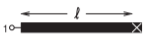
Figure \(\PageIndex{16}\): A \(50\:\Omega\) shorted gold microstrip line with width \(w = 500\:\mu\text{m}\), length \(\ell = 1\text{ cm}\) on a \(600\:\mu\text{m}\) thick alumina substrate with relative permittivity \(\varepsilon_{r} = 9.8\) and loss tangent \(\tan\delta = 0.001\).

3.4.5 An Alternative Admittance Chart

Design often requires switching between admittance and impedance. So it is convenient to use the colored combined Smith chart shown in Figure \(\PageIndex{9}\). Monochrome charts were once the only ones available and an impedance Smith chart was used for admittance-based calculations provided that reflection coefficients are rotated by \(180^{\circ}\). This form of the Smith chart is not used now.

3.4.6 Expanded Smith Chart

Another form of the Smith chart is the expanded Smith chart shown in Figure 3.5.1. This is used to plot reflection coefficients of loads with a negative resistance that have a reflection coefficient magnitude greater than one. An oscillator, for example, presents a negative resistance to a resonator. It is also used to plot transmission parameters that have a magnitude greater than one, such as the forward transmission parameter, \(S_{21}\), of a transistor.

3.4.7 Summary

The Smith chart is the most powerful of tools used in RF and Microwave Design. Design using Smith charts will be considered in other chapters but at this stage the reader should be totally conversant with the techniques described in this section.

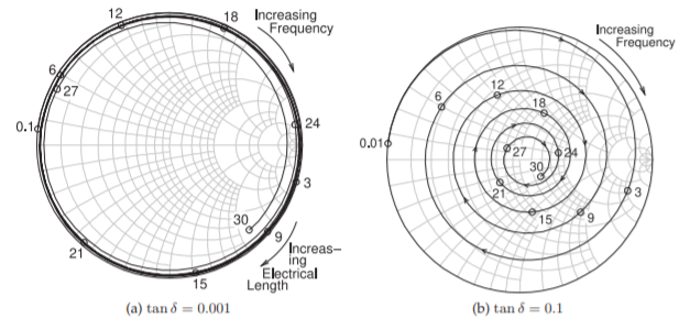
Figure \(\PageIndex{17}\): Smith chart plot of the reflection coefficient of the shorted \(1\text{ cm}\)-long microstrip line in Figure \(\PageIndex{16}\): (a) a low-loss substrate with \(\tan\delta = 0.001\); and (b) a high-loss substrate with \(\tan\delta = 0.1\). Frequencies are marked in gigahertz.