5.2: \(Q\) Factor

RF inductors and capacitors also have loss and parasitic elements. With inductors there is both series resistance and shunt capacitance mainly from interwinding capacitance, while with capacitors there will be shunt resistance and series inductance. A practical inductor or capacitor is limited

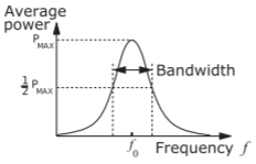
Figure \(\PageIndex{1}\): Transfer characteristic of a resonant circuit. (The transfer function is \(V/I\) for the parallel resonant circuit of Figure \(\PageIndex{2}\)(a) and \(I/V\) for the series resonant circuit of Figure \(\PageIndex{2}\)(b).)

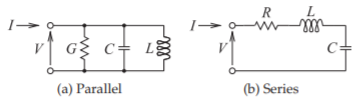
Figure \(\PageIndex{2}\): Second-order resonant circuits.

to operation below the self-resonant frequency determined by the inductance and capacitance itself resonating with its reactive parasitics. The impact of loss is quantified by the \(Q\) factor (the quality factor). \(Q\) is loosely related to bandwidth in general and the strict relationship is based on the response of a series or parallel connection of a resistor (\(R\)), an inductor (\(L\)), and a capacitor (\(C\)). The response of an \(RLC\) network is described by a second-order differential equation with the conclusion that the \(3\text{ dB}\) fractional bandwidth of the response (i.e., when the power response is at its half-power level below its peak response) is \(1/Q\). (The fractional bandwidth is \(\Delta f /f_{0}\) where \(f_{0} = f_{r}\) is the resonant frequency at the center of the band and \(\Delta f\) is the \(3\text{ dB}\) bandwidth.) This is not true for any network other than a second-order circuit, but as a guiding principle, networks with higher \(Q\)s will have narrower bandwidths.

5.2.1 Definition

The \(Q\) factor of a component at frequency \(f\) is defined as the ratio of \(2\pi f\) times the maximum energy stored to the energy lost per cycle. In a lumped-element resonant circuit, stored energy is transferred between an inductor, which stores magnetic energy, and a capacitor, which stores electric energy, and back again every period. Distributed resonators function the same way, exchanging energy stored in electric and magnetic forms, but with the energy stored spatially. The quality factor is

\[\label{eq:1}Q=2\pi f_{r}\left(\frac{\text{average energy stored in the resonator at }f_{r}}{\text{power lost in the resonator}}\right) \]

where \(f_{1} = \omega_{r}/(2π)\) is the resonant frequency.

A simple response is shown in Figure \(\PageIndex{1}\). For a parallel resonant circuit with elements \(L,\: C,\) and \(G = 1/R\) (see Figure \(\PageIndex{2}\)(a)),

\[\label{eq:2}Q=\omega_{r}C/G=1/(\omega_{r}LG) \]

where \(f_{r} = \omega_{r}/(2π)\) is the resonant frequency and is the frequency at which the maximum amount of energy is stored in a resonator. The conductance, \(G\), describes the energy lost in a cycle. For a series resonant circuit (Figure \(\PageIndex{2}\)(b)) with \(L,\: C,\) and \(R\) elements,

\[\label{eq:3}Q=\omega_{r}L/R=1/(\omega_{r}CR) \]

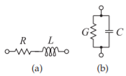
Figure \(\PageIndex{3}\): Loss elements of practical inductors and capacitors: (a) an inductor has a series resistance \(R\); and (b) for a capacitor, the dominant loss mechanism is a shunt conductance \(G = 1/R\).

These second-order resonant circuits have a bandpass transfer characteristic (see Figure \(\PageIndex{1}\)) with \(Q\) being the inverse of the fractional bandwidth of the resonator. The fractional bandwidth, \(\Delta f /f_{r}\), is measured at the half-power points as shown in Figure \(\PageIndex{1}\). (\(\Delta f\) is also referred to as the two-sided \(−3\text{ dB}\) bandwidth.) Then

\[\label{eq:4}Q=f_{r}/\Delta f \]

Thus the \(Q\) is a measure of the sharpness of the bandpass frequency response. The determination of \(Q\) using the measurement of bandwidth together with Equation \(\eqref{eq:4}\) is often not very precise, so another definition that uses the much more sensitive phase change at resonance is preferred when measurements are being used. With \(\phi\) being the phase (in radians) of the transfer characteristic, the definition of \(Q\) is now

\[\label{eq:5}Q=\frac{\omega_{r}}{2}\left|\frac{d\phi}{d\omega}\right| \]

Equation \(\eqref{eq:5}\) is another equivalent definition of \(Q\) for parallel \(RLC\) or series \(RLC\) resonant circuits. It is meaningful to talk about the \(Q\) of circuits other than three-element \(RLC\) circuits, and then its meaning is always a ratio of the energy stored to the energy dissipated per cycle. The \(Q\) of these structures can no longer be determined by bandwidth or by the rate of phase change.

5.2.2 \(Q\) of Lumped Elements

\(Q\) is also used to characterize the loss of lumped inductors and capacitors. Inductors have a series resistance \(R\), and the main loss mechanism of a capacitor is a shunt conductance \(G\) (see Figure \(\PageIndex{3}\)).

The \(Q\) of an inductor at frequency \(f =\omega /(2\pi )\) with a series resistance \(R\) and inductance \(L\) is

\[\label{eq:6}Q_{\text{INDUCTOR}}=\frac{\omega L}{R} \]

Since \(R\) is approximately constant with respect to frequency for an inductor, the \(Q\) will vary with frequency.

The \(Q\) of a capacitor with a shunt conductance \(G\) and capacitance \(C\) is

\[\label{eq:7}Q_{\text{CAPACITOR}}=\frac{\omega C}{G} \]

\(G\) is due mainly to relaxation loss mechanisms of the dielectric of a capacitor and so varies linearly with frequency. Thus the \(Q\) of a capacitor is almost constant with respect to frequency. For microwave components invariably \(Q_{\text{CAPACITOR}} ≫ Q_{\text{INDUCTOR}}\), and \(Q_{\text{INDUCTOR}}\) is smaller than the \(Q\) of transmission line networks. Thus, if the length of a transmission line is not too long, transmission line networks are preferred. If lumped elements must be used, the use of inductors should be minimized.

5.2.3 Loaded \(Q\) Factor

The \(Q\) of a component as defined in the previous section is called the unloaded \(Q,\: Q_{U}\). However if a component is to be measured or used in any way, it is necessary to couple energy in and out of it. The \(Q\) is reduced and thus the resonator bandwidth is increased by the power lost to the external circuit so that the loaded \(Q\), then the loaded \(Q\) is

\[\begin{align}Q_{L}&=2\pi f_{0}\left(\frac{\text{average energy stored in the resonator at }f_{0}}{\text{power lost in the resonator and to the external circuit}}\right)\nonumber \\ \label{eq:8}&=\frac{1}{1/Q+1/Q_{X}}\end{align} \]

where \(Q_{X}\) is called the external \(Q\). \(Q_{L}\) accounts for the power extracted from the resonant circuit.

So a parallel \(LCG\) circuit with elements \(L_{r},\: C_{r},\) and \(G_{r}\) (at resonance) loaded by a shunt conductance \(G_{l}\) has

\[\label{eq:9}Q_{U}=\omega_{r}C_{r}/G_{r}=1/(\omega_{r}L_{r}G_{r}) \]

and

\[\label{eq:10}Q_{L}=\omega_{r}C_{r}/(G_{r}+G_{l}) \]

Thus

\[\label{eq:11}\frac{1}{Q_{L}}=\frac{1}{Q_{U}}+\frac{1}{Q_{X}} \]

or

\[\label{eq:12}Q_{X}=\left(\frac{1}{Q_{L}}-\frac{1}{Q_{U}}\right)^{-1} \]

\(Q_{X}\) is called the external \(Q\), and it describes the effect of loading. \(Q_{L}\) is the \(Q\) that would actually be measured. \(Q_{U}\) normally needs to be determined, but if the loading is kept very small, \(Q_{L}\approx Q_{U}\).

5.2.4 Summary of the Properties of \(Q\)

In summary:

1. \(Q\) is properly defined and related to the energy stored in a resonator for a second-order network, one with two reactive elements of opposite types.
2. \(Q\) is not well defined for networks with three or more reactive elements.
3. However, \(Q\) is a frequently used parameter in the design equations for more complex networks than second-order ones.
4. For complex networks the \(Q\) is defined as the ratio of a reactance to a resistance when looking into one end of the network at one frequency. This value of \(Q\) should not be used to deduce the bandwidth of the network.
5. It is only used (as defined or some approximation of it) for guiding the design.