5.6: Transmission Line Stubs and Discontinuities

Interruptions of the magnetic or electric field create regions where additional magnetic energy or electric energy is stored. If the additional energy stored is predominantly magnetic, the discontinuity will introduce an inductance. If the additional energy stored is predominantly electric, the discontinuity will introduce a capacitance. Such discontinuities occur with all transmission lines. In some cases transmission line discontinuities introduce undesired parasitics, but they also provide an opportunity to effectively introduce lumped-element components. In this section microstrip discontinuities will be considered, but the principles apply to all transmission line structures. The simplest microwave circuit element is a uniform section of transmission line that can be used to introduce a time delay or frequency-dependent phase shift. More commonly it is used to interconnect other components. Line segments including bends and junctions are shown in Figure \(\PageIndex{1}\).

5.6.1 Open

Many transmission line discontinuities arise from fringing fields. One element is the microstrip open, shown in Figure \(\PageIndex{2}\). The fringing fields at the end of the transmission line in Figure \(\PageIndex{2}\)(a) store energy in the electric field, and this can be modeled by the fringing capacitance, \(C_{F}\), shown in Figure \(\PageIndex{2}\)(b). This effect can also be modeled by an extended transmission line, as shown in Figure \(\PageIndex{2}\)(c). For a typical microstrip line with \(\varepsilon_{r} = 9.6,\: h = 600\:\mu\text{m},\) and \(w/h = 1,\) \(C_{F}\) is approximately \(36\text{ fF}\). However, \(C_{F}\) varies with frequency, and the extended length is a much better approximation to the effect of fringing [12]. For the same dimensions, the length of the extension is approximately \(0.35h\) and almost independent of frequency [13]. As with many fringing effects, a capacitance or inductance can be used to model the effect of fringing, but generally a distributed model is better.

5.6.2 Discontinuities

Several microstrip discontinuities and their equivalent circuits are shown in Figure \(\PageIndex{3}\). Discontinuities (Figure \(\PageIndex{3}\)(b–g)) are modeled by capacitive elements if the \(E\) field is affected and by inductive elements if the \(H\) field (or current) is disturbed. The stub shown in Figure \(\PageIndex{3}\)(b), for example, is best modeled using lumped elements describing the junction as well as the transmission line of the stub itself. Current bunches at the right angle bends from the through line to the stub. The current bunching leads to excess energy being stored in the magnetic field, and hence an inductive effect. There is also excess charge storage in the parallel plate region bounded by the left- and right-hand through lines and the stub. This is modeled by a capacitance.

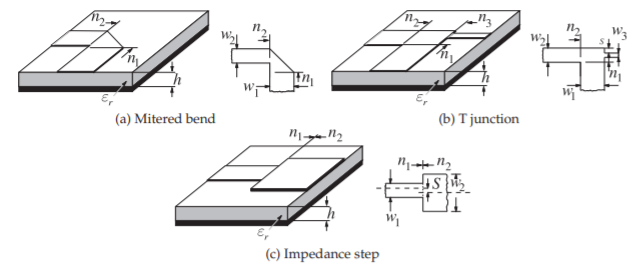
Figure \(\PageIndex{1}\): Microstrip discontinuities.

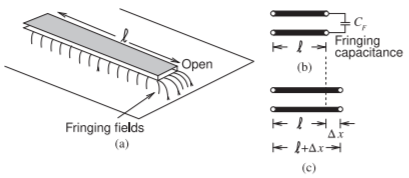
Figure \(\PageIndex{2}\): An open on a microstrip transmission line: (a) microstrip line showing fringing fields at the open; (b) fringing capacitance model of the open; and (c) an extended line model of the open with \(\Delta x\) being the extra transmission line length that captures the open.

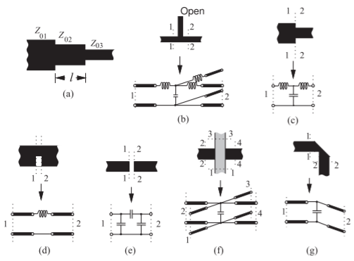
Figure \(\PageIndex{3}\): Microstrip discontinuities: (a) quarter-wave impedance transformer; (b) open microstrip stub; (c) step; (d) notch; (e) gap; (f) crossover; and (g) bend.

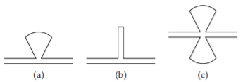
Figure \(\PageIndex{4}\): Microstrip stubs: (a) radial shunt-connected stub; (b) conventional shunt stub; and (c) butterfly radial stub.

5.6.3 Impedance Transformer

Impedance transformers interface two lines of different characteristic impedance. The smoothest transition and the one with the broadest bandwidth is a tapered line. This element can be long and then a quarter-wave impedance transformer (see Figure \(\PageIndex{3}\)(a)) is sometimes used, although its bandwidth is relatively small and centered on the frequency at which \(l = \lambda_{g}/4\). Ideally \(Z_{0,2} =\sqrt{Z_{0,1}Z_{0,3}}\). This topic is considered further in Section 7.5 where the design of tapered lines and multi-stage quarter-wave transformers are considered in detail.

5.6.4 Planar Radial Stub

The use of a radial stub (Figure \(\PageIndex{4}\)(a)), as opposed to the conventional microstrip stub (Figure \(\PageIndex{4}\)(b)), can improve the bandwidth of many microstrip circuits. A major advantage of a radial stub is that the input impedance presented to the through line generally has broader bandwidth than that obtained with the conventional stub. When two shunt-connected radial stubs are introduced in parallel (i.e., one on each side of the microstrip feeder line) the resulting configuration is termed a “butterfly” stub (see Figure \(\PageIndex{4}\)(c)). Critical design parameters include the radius, \(r\), and the angle of the stub.

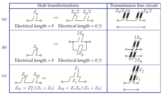
Figure \(\PageIndex{5}\): Stub network transformations: (a) open- and (b) short-circuited stubs after application of the half-angle transform [14]; and (c) equivalence between series connection of open- and short-circuited stubs and stepped impedance transmission line.

5.6.5 Stub Transformations

The stub transformations in Figure \(\PageIndex{5}\) enable the lengths of stubs to be reduced. The first two stub transformations (Figure \(\PageIndex{5}\)(a and b)) are called half-angle transformations and enable a stub to be replaced by two shorter stubs. The third stub transformation (Figure \(\PageIndex{5}\)(c)) enables two stubs to be replaced by two cascaded transmission lines.

Figure \(\PageIndex{5}\)(a) is a half-angle transform of a series open-circuited stub. Mathematically the transform is described as follows. Consider the input impedance of an open-circuited stub [14] with electrical length \(\theta = \beta\ell\) at frequency \(f\) and which is a quarter-wavelength long at \(f_{0}\) (i.e., \(\theta = \pi/2\) at \(f_{0}\)) (from Section 2.4.4 of [15] and using Equation ((1.105)) of [15]):

\[\label{eq:1} Z_{oc}=-\jmath Z_{0}\cot (\theta )=\jmath (Z_{0}/2)\tan(\theta/2)-\jmath (Z_{0}/2)\tan(\theta /2) \]

In general,\(\theta = (\pi /2)\) \((f/f_{0})\). The right-hand side of Equation \(\eqref{eq:1}\) describes the series connection of short- and open-circuited stubs having characteristic impedances of \(Z_{0}/2\) and half the original electrical length. This implies that the resulting transmission line resonators are one-quarter wavelength long at \(2f_{0}\) (i.e., they are one-eighth wavelength long at \(f_{0}\)). The half-angle transformation applies at all frequencies and not just frequencies near \(f_{0}\). Through a similar analytical treatment, the short-circuited stub has the equivalence shown in Figure \(\PageIndex{5}\)(b). The series short-circuited stub on the left in Figure \(\PageIndex{5}\)(b) has the series admittance

\[\label{eq:2}Y_{T}=\frac{1}{\jmath Z_{0}\tan(\theta )}=\frac{1}{\jmath Z_{0}}\cot (\theta ) \]

and the stubs in the transformation have an input impedance

\[\label{eq:3}Z_{oc}=-\jmath\frac{1}{2}Z_{0}\cot(\theta /2)\quad\text{and}\quad Z_{sc}=\jmath\frac{1}{2}Z_{0}\tan(\theta /2) \]

These stubs are in parallel so that the total input admittance is

\[\begin{align}Y_{T}&=\frac{1}{Z_{oc}}+\frac{1}{Z_{sc}}=\frac{2}{-\jmath Z_{0}\cot(\theta /2)}+\frac{1}{\jmath Z_{0}\tan (\theta /2)}\nonumber \\ \label{eq:4} &=\frac{2}{\jmath Z_{0}}\left[-\tan(\theta /2)+\cot (\theta /2)\right]=\frac{1}{\jmath Z_{0}}\cot(\theta )\end{align} \]

Examining Equations \(\eqref{eq:2}\) and \(\eqref{eq:4}\) it is seen that they are identical, thus Figure \(\PageIndex{5}\)(b) represents another half-angle transformation.

For the series open- and short-circuited stubs in Figure \(\PageIndex{5}\)(c), the input impedances of the open- and short-circuited stubs are

\[\label{eq:5}Z_{oc}=-\jmath Z_{02}\cot(\theta)\quad\text{and}\quad Z_{sc}=\jmath Z_{01}\tan(\theta ) \]

respectively, so that the total series impedance is

\[\label{eq:6}Z_{T}=Z_{oc}+Z_{sc}=-\jmath Z_{02}\cot (\theta)+\jmath Z_{01}\tan (\theta) \]

For the transformation on the right, the impedance looking into the open circuit (outer) stub is

\[\label{eq:7}Z_{x}=-\jmath Z_{2}\cot (\theta) \]

and the total impedance is

\[\label{eq:8}Z_{T}=Z_{1}\left[\frac{−\jmath Z_{2} \cot(\theta) + \jmath Z_{1} \tan(\theta )}{Z_{1} + Z_{2} \cot(\theta )\tan(\theta )}\right]=\frac{−\jmath Z_{1}Z_{2} \cot(\theta )}{Z_{1}+Z_{2}}+\frac{\jmath Z_{1}^{2}\tan(\theta)}{Z_{1}+Z_{2}} \]

Equating Equations \(\eqref{eq:6}\) and \(\eqref{eq:8}\) and collecting terms,

\[\label{eq:9}Z_{02}=Z_{1}Z_{2}/(Z_{1}+Z_{2})\quad\text{and}\quad Z_{01}=Z_{1}^{2}/(Z_{1}+Z_{2}) \]

and the transmission line segments (of characteristic impedance \(Z_{01},\: Z_{02},\: Z_{1}\) and \(Z_{2}\)) all have the same electrical length.

In summary, the stub transformations hold no matter what the lengths of the stubs. The half-angle stub transformations enable transmission line circuits to be miniaturized.