2.7: Models of Transmission Lines
- Page ID
- 41021
Models of transmissions lines enable lines to be incorporated in simulators and related to lumped-element circuits. Section 2.7.1 presents models used in circuit simulators such as Spice. Synthesis of microwave circuits often requires that a lumped-element design be realized using an equivalent transmission line network. The ABCD parameter technique described in Section 2.7.2 is the main means for relating these networks and thus synthesizing transmission line-based designs. This method is used many times in designs in this book series.
2.7.1 Circuit Models of Transmission Lines
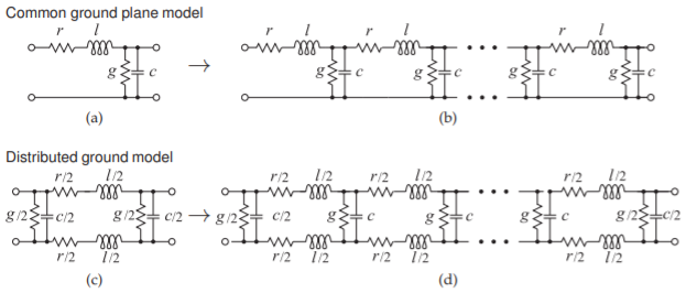
Circuit models of transmission lines are required if they are to be used in a circuit simulator. RF and microwave engineering uses two types of simulators. Spice-like simulators use lumped-element transmission line models in which an \(RLGC\) model of a short segment of line is replicated for the length of the line. If the ground plane is treated as a universal ground, then the model of a segment of length \(\Delta z\) is as shown in Figure \(\PageIndex{1}\)(a). In this segment \(r = R\Delta z,\: l = L\Delta z,\: g = G\Delta z,\) and \(c = C\Delta ∆z\), where \(R,\: L,\: G,\) and \(C\) are the per unit length parameters of the line. Cascading the segments to get the length of the line yields the complete lumped-element model of the line, as shown in Figure \(\PageIndex{1}\)(b). This model is adequate if there is a well-defined ground plane. Otherwise the more accurate form of the segment model shown in Figure \(\PageIndex{1}\)(c) is used. The \(L\) and \(C\) of a two-conductor transmission line model relate to the fields between the conductors and not to the conductors themselves. So assigning them to just one conductor is not accurate. The capacitor is already shared between the two conductors in the original model, Figure \(\PageIndex{1}\)(a), but the inductor was assigned to just one. The change in the distributed ground model of Figure \(\PageIndex{1}\)(c) is that inductance

Figure \(\PageIndex{1}\): Lumped-element transmission line models: (a) model of a short segment (e.g. \(\lambda/20\) long); (b) complete model of a transmission line; (c) more accurate model of a segment; and (d) complete accurate model of a transmission line.
is assigned to each of the conductors.
One of the problems with the lumped-element model is that it is not possible to handle \(G\) correctly. \(G\) is largely due to dielectric relaxation loss and so is linearly dependent on frequency. Fortunately it is very small for RF and microwave substrates and so it can nearly always be ignored. An exception is a silicon integrated circuit where there is appreciable dielectric loss. Parasitic extraction software is used in silicon integrated circuit design to extract models similar to that in Figure \(\PageIndex{1}\)(d) but account for coupling with other circuits. Especially in digital circuits, it is sometimes difficult to identify a ground plane (a current return path) except for critical interconnect networks such as clock and power distribution circuits.
Communication filters are often constructed using several shorted transmission line resonators that are coupled to each other. Consider a coaxial line that is short-circuited at one end. The permittivity filling the coaxial line has \(\varepsilon = 20\) and the resonator is to be designed to resonate at a center frequency, \(f_{0}\), of \(1850\text{ MHz}\) when it is \(\lambda/4\) long.
- What is the wavelength in the dielectric-filled coaxial line?
- What is the form of the equivalent circuit (in terms of inductors and capacitors) of the one-quarter wavelength long resonator if the coaxial line is lossless? Note that the input impedance of a shorted \(\lambda/4\)-long line is infinite.
- What is the physical length of the resonator?
Solution
The first thing to realize with this example is that the first resonance will occur when the length of the resonator is one-quarter wavelength \((\lambda/4)\) long. Resonance generally means that the impedance is either an open or a short circuit and there is energy stored. When the shorted line is \(\lambda/4\) long, the input impedance is an open circuit and also energy is stored.
- \(\lambda_{g} = \lambda_{0}/\sqrt{\varepsilon_{r}} = 16.2\text{ cm}/\sqrt{20} = 3.62\text{ cm}\). (Here \(\lambda_{0} = 30\text{ cm}\) at \(1\text{ GHz}\) was used. Thus at \(1850\text{ MHz}\) \(\lambda_{0} = (30\text{ cm})/1.85 = 16.2\text{ cm}\).)
-

Figure \(\PageIndex{2}\)
\(Y=0\) at resonance
\(Y=Y_{L}+Y_{C}=\frac{1}{\jmath\omega L}+\jmath\omega C=\frac{\omega^{-1}}{\jmath L}+\jmath\omega C\) - \(\ell =(0.0362\text{ m})/4=9.05\text{ mm}\)
This example builds on Example \(\PageIndex{1}\). RF communication filters are often constructed using several shorted transmission line resonators that are coupled to each other. Consider a coaxial line that is short-circuited at one end. The dielectric filling the coaxial line has a \(\varepsilon = 20\) and the resonator is to be designed to resonate at a center frequency \(f_{0} = 1850\text{ MHz}\).
- What is the wavelength in the dielectric-filled coaxial line?
- What is the form of the equivalent circuit (in terms of inductors and capacitors) of the one-quarter wavelength long resonator if the coaxial line is lossless?
- What is the physical length of the resonator?
- Determine the derivative with respect to frequency of the admittance of the \(LC\) equivalent circuit developed in (b). Determine an analytic expression for the derivative at the resonant frequency.
- If the diameter of the inner conductor of the coaxial line is \(2\text{ mm}\) and the inside diameter of the outer conductor is \(5\text{ mm}\), what is the characteristic impedance of the coaxial line?
- Calculate the input admittance of the dielectric-filled coaxial line at \(0.99f_{0},\: f_{0},\) and \(1.01f_{0}\). Determine the numerical frequency derivative of the line admittance at \(f_{0}\).
- Derive the numeric values of the equivalent circuit of the resonator at resonance.
Solution
The first thing to realize is that the first resonance will occur when the length of the resonator is one-quarter wavelength \((\lambda/4)\) long. Resonance generally means that the impedance is either an open or a short circuit and there is energy stored. When the shorted line is \(\lambda/4\) long, the input impedance will be an open circuit. When the line is of zero length energy is not stored, so a zero-length line is not a resonator.
- \(\lambda_{g} =\lambda_{0}/\sqrt{\varepsilon_{r}} = 16.2\text{ cm}/\sqrt{20} = 3.62\text{ cm}\).
-

Figure \(\PageIndex{3}\)
\(Y=Y_{L}+Y_{C}=\frac{1}{\jmath\omega L}+\jmath\omega C=\frac{\omega^{-1}}{\jmath L}+\jmath\omega C\).
\(Y=0\) at resonance. - \(\ell = (0.0362\text{ m})/4 = 9.05\text{ mm}\).
- From (b),
\[\label{eq:1}\frac{\partial Y}{\partial\omega}=-\frac{\omega^{-2}}{\jmath L}+\jmath C=\frac{\jmath}{\omega^{2}L}+\jmath C=\jmath\left(\frac{1}{\omega^{2}L}+C\right) \] - From Equation (2.2.50), \(Z_{0} = 12.28\:\Omega\).
- \(Z_{L} =0\:\Omega,\:\ell = (0.0362\text{ m})/4=9.05\text{ mm},\:\beta =\beta_{0}\sqrt{\varepsilon_{r}},\) where \(\beta_{0}\)β0 is the phase constant of free space. From Equations (2.2.40) and (2.2.41),
\[\beta=20.958\times f_{0}|_{\text{GHz}}\times\sqrt{20}=173.4\text{ rad/m}\nonumber \]
At \(0.99\:f_{0}\) and using Equation (2.3.18), \(Z_{\text{in}} = \jmath 781.7\:\Omega;\: Y_{\text{in}} = −\jmath 0.001279\text{ S}\).
At \(f_{0},\: Z_{\text{in}} = −\jmath\infty\:\Omega;\: Y_{\text{in}} = 0\text{ S}\). At \(1.01\:f_{0},\: Z_{\text{in}} = −\jmath 781.7\:\Omega;\: Y_{\text{in}} = \jmath 0.001279\text{ S}\).
So the derivative of the input admittance is
\[\label{eq:2}\frac{\partial Y}{\partial\omega}\approx\frac{\Delta Y_{\text{in}}}{\Delta\omega}=\frac{\jmath(0.001279+0.001279)}{2\pi f_{0}(1.01-0.99)}=\jmath 1.101\cdot 10^{-11}\text{ S}\cdot\text{s}=\jmath 1.101\cdot 10^{-11}\text{ F} \]
Note the SI unit equivalence \(\text{S}\cdot\text{s} = \text{F}\) obtained by examining Table 2.A.1. - The LC circuit resonates at \(f_{0} = 1.85\text{ GHz}\) when \(1/(\jmath\omega_{0}L) = −\jmath\omega_{0}C;\: \omega_{0}= 2\pi f_{0}\). Thus
\[\label{eq:3}LC=\omega_{0}^{-2}=0.7401\times 10^{-20}\text{ s}^{2} \]
Equating Equations \(\eqref{eq:1}\) and \(\eqref{eq:2}\):
\[\label{eq:4}\frac{1}{\omega_{0}^{2}L}+C=1.101\times 10^{-11}\text{ F}\quad\text{ and so }\quad C=1.101\times 10^{-11}-\frac{1}{\omega_{0}^{2}L}\text{ F} \]
Substituting this in Equation \(\eqref{eq:3}\) (noting the SI unit equivalence \(\text{S}^{−1}\cdot\text{s}^{-1}=\text{H}\):
\[L\left(1.101\times 10^{-11}-\frac{1}{\omega_{0}^{2}L}\right)=0.7401\times 10^{-20}\text{ H}\nonumber \]
\[\label{eq:5} 1.101 \times 10^{−11}L = 1.4802\times 10^{−20}\text{ H}\quad\text{and}\quad L = 1.345\times 10^{−9}\text{ H} = 1.345\text{ nH} \]
From Equation \(\eqref{eq:4}\),
\[\label{eq:6}C=0.7401\times 10^{-20}/L=5.503\times 10^{-12}\text{ F}=5.503\text{ pF} \]
So the equivalent circuit of the resonator is

Figure \(\PageIndex{4}\)
with \(L = 1.345\text{ nH}\) and \(C = 5.503\text{ pF}\).
This equivalent circuit is valid for a range (say \(5\%– 10\%\)) of frequencies around \(1.85\text{ GHz}\). The broadband equivalence was obtained here by matching both the admittance and the derivative of the admittance.

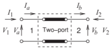
Figure \(\PageIndex{5}\): Two-port network of a transmission line with cascadable voltage and current definitions.
2.7.2 \(ABCD\) (Chain) Parameters of a Transmission Line
\(ABCD\) parameters, also called chain parameters, are used in RF and microwave engineering to electrically equate two different structures such as a lumped-element network and a transmission line structure. Often the electrical design is undertaken using lumped elements and then these are converted to equivalent transmission line structures with the equivalence achieved using \(ABCD\) parameters.
Figure \(\PageIndex{5}\), shows the voltages and currents of a two-port in cascadable form so that the input variables can be written in terms of the output variables:
\[\label{eq:7}\left[\begin{array}{c}{V_{a}}\\{I_{a}}\end{array}\right]=\left[\begin{array}{cc}{A}&{B} \\ {C}&{D}\end{array}\right]\left[\begin{array}{c}{V_{b}}\\{I_{b}}\end{array}\right] \]
Note that the current at port 2 is in the opposite direction to the usual definition of the two-port current. So in terms of the port voltage and current at port 1, (\(V_{1}\) and \(I_{1}\)), and the port voltage and current at port 2, (\(V_{2}\) and \(I_{2}\)),
\[\label{eq:8}V_{a}=V_{1},\quad I_{a}=I_{1},\quad V_{b}=V_{2},\quad\text{and}\quad I_{b}=-I_{2} \]
In terms of traveling-wave voltages, the total voltage and current on a line of length \(\ell\), propagation constant \(\gamma\), and characteristic impedance \(Z_{0} = 1/Y_{0}\) at position \(z\) are
\[\begin{align}\label{eq:9}V(z)&=V_{0}^{+}e^{-\jmath\gamma(z-\ell)}+V_{0}^{-}e^{\jmath\gamma(z-\ell)} \\ \label{eq:10}I(z)&=Y_{0}V_{0}^{+}e^{-\jmath\gamma(z-\ell)}-Y_{0}V_{0}^{-}e^{\jmath\gamma(z-\ell)}\end{align} \]
where \(V_{0}^{+}\) and \(V_{0}^{-}\) are the traveling wave voltage phasors at \(z =\ell\), (port 2), i.e.
\[\label{eq:11}V_{0}^{+}=\frac{1}{2}(V_{2}+Z_{0}I_{2})\quad\text{and}\quad V_{0}^{-}=\frac{1}{2}(V_{2}-Z_{0}I_{2}) \]
Substituting these into Equations \(\eqref{eq:9}\) and \(\eqref{eq:10}\),
\[\begin{align}\label{eq:12}V(z)&=\frac{1}{2}(V_{2}+Z_{0}I_{2})e^{-\jmath\gamma(z-\ell)}+\frac{1}{2}(V_{2}-Z_{0}I_{2})e^{\jmath\gamma(z-\ell)} \\ \label{eq:13}I(z)&=\frac{1}{2}(Y_{0}V_{2}+I_{2})e^{-\jmath\gamma(z-\ell)}-\frac{1}{2}(Y_{0}V_{2}-I_{2})e^{\jmath\gamma(z-\ell)}\end{align} \]
At Port 1 \((z = 0)\)
\[\begin{align}\label{eq:14}V_{1}=V(0)&=\frac{1}{2}(V_{2}+Z_{0}I_{2})e^{\jmath\gamma\ell}+\frac{1}{2}(V_{2}-Z_{0}I_{2})e^{-\jmath\gamma\ell} \\ \label{eq:15}I_{1}=I(0)&=\frac{1}{2}(Y_{0}V_{2}+I_{2})e^{\jmath\gamma\ell}-\frac{1}{2}(Y_{0}V_{2}-I_{2})e^{-\jmath\gamma\ell}\end{align} \]

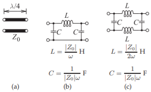
Figure \(\PageIndex{6}\): Lumped equivalent circuit of a one-quarter wavelength long line of characteristic impedance \(Z_{0}\) which is the same as that of an impedance inverter (of \(Z_{0}\:\Omega\)): (a) one-quarter wavelength long line segment; (b) lumped-element equivalent circuit; and (c) alternative lumped-element model.
Using the trigonometric identities in Section 1.A.2 (and noting that \(I_{2} = −I_{b}\)),
\[\begin{align}\label{eq:16}V_{a}&=V_{1}=\cosh(\gamma\ell)V_{2}-Z_{0}\sinh(\gamma\ell)I_{2}=\cosh(\gamma\ell)V_{b}+Z_{0}\sinh(\gamma\ell)I_{b} \\ \label{eq:17}I_{a}&=I_{1}=Y_{0}\sinh(\gamma\ell)V_{2}-\cosh(\gamma\ell)I_{2}=Y_{0}\sinh(\gamma\ell)V_{b}+\cosh(\gamma\ell)I_{b}\end{align} \]
That is, the \(ABCD\) parameters of a lossy line are
\[\begin{align}A&=\cosh(\gamma\ell) &B&=Z_{0}\sinh(\gamma\ell)\nonumber \\ \label{eq:18}C&=Y_{0}\sinh(\gamma\ell) &D&=\cosh(\gamma\ell)\end{align} \]
and the \(ABCD\) parameters of a lossless transmission line, where \(\gamma=\jmath\beta\), are
\[\begin{align}A&=\cos(\beta\ell) &B&=\jmath Z_{0}\sin(\beta\ell) \nonumber \\ \label{eq:19}C&=\jmath Y_{0}\sin(\beta\ell) &D&=\cos(\beta\ell)\end{align} \]
Develop the lumped-element model of a one-quarter wavelength long lossless transmission line having characteristic impedance \(Z_{0}\).
Solution
The model is developed by equating \(ABCD\) parameters. The \(ABCD\) parameters of a onequarter wavelength long lossless line (with \(\beta\ell = \pi/2\)) are
\[\begin{align}\label{eq:20}A&=\cos(\beta\ell)=0 \\ \label{eq:21}B&=\jmath Z_{0}\sin(\beta\ell)=\jmath Z_{0} \\ \label{eq:22}C&=\jmath Y_{0}\sin(\beta\ell)=\jmath /Z_{0} \\ \label{eq:23} D&=\cos(\beta\ell)=0\end{align} \]
The \(ABCD\) parameters of a Pi network (see Table 2.A.1 of [7]) are
\[\begin{align}\label{eq:24}A&=1+y_{2}/y_{3} \\ \label{eq:25} B&=1/y_{3} \\ \label{eq:26}C&=y_{1}+y_{2}+y_{1}y_{2}/y_{3} \\ \label{eq:27}D&=1+y_{1}/y_{3}\end{align} \]
Equating Equations \(\eqref{eq:21}\) and \(\eqref{eq:25}\),
\[\label{eq:28}y_{3}=1/(\jmath Z_{0}) \]
and with Equations \(\eqref{eq:20}\), \(\eqref{eq:23}\), \(\eqref{eq:24}\), and \(\eqref{eq:27}\),
\[\label{eq:29}y_{1}=y_{2}=-y_{3}=-1/(\jmath Z_{0}) \]
The lumped equivalent circuit of the quarter-wave transformer in Figure \(\PageIndex{6}\)(a) is shown in Figure \(\PageIndex{6}\)(b). An alternative lumped-element model is shown in Figure \(\PageIndex{6}\)(c). The lumped-element model of the \(50\:\Omega\) line at \(400\text{ MHz}\) is shown in Figure \(\PageIndex{6}\)(b) with \(L = 19.89\text{ nH}\) and \(C = 7.968\text{ pF}\). This is a simpler and more accurate model of a \(\lambda/4\) long line than a model with multiple short line segments as in Figure \(\PageIndex{1}\).


