2.10: Cascaded Line Realization of Filters

Last updated
Save as PDF

Page ID: 46068

\( \newcommand{\vecs}[1]{\overset { \scriptstyle \rightharpoonup} {\mathbf{#1}} } \) \( \newcommand{\vecd}[1]{\overset{-\!-\!\rightharpoonup}{\vphantom{a}\smash {#1}}} \)\(\newcommand{\id}{\mathrm{id}}\) \( \newcommand{\Span}{\mathrm{span}}\) \( \newcommand{\kernel}{\mathrm{null}\,}\) \( \newcommand{\range}{\mathrm{range}\,}\) \( \newcommand{\RealPart}{\mathrm{Re}}\) \( \newcommand{\ImaginaryPart}{\mathrm{Im}}\) \( \newcommand{\Argument}{\mathrm{Arg}}\) \( \newcommand{\norm}[1]{\| #1 \|}\) \( \newcommand{\inner}[2]{\langle #1, #2 \rangle}\) \( \newcommand{\Span}{\mathrm{span}}\) \(\newcommand{\id}{\mathrm{id}}\) \( \newcommand{\Span}{\mathrm{span}}\) \( \newcommand{\kernel}{\mathrm{null}\,}\) \( \newcommand{\range}{\mathrm{range}\,}\) \( \newcommand{\RealPart}{\mathrm{Re}}\) \( \newcommand{\ImaginaryPart}{\mathrm{Im}}\) \( \newcommand{\Argument}{\mathrm{Arg}}\) \( \newcommand{\norm}[1]{\| #1 \|}\) \( \newcommand{\inner}[2]{\langle #1, #2 \rangle}\) \( \newcommand{\Span}{\mathrm{span}}\)\(\newcommand{\AA}{\unicode[.8,0]{x212B}}\)

In this section, filters are presented that use cascaded sections of transmission line, realizing series inductors and shunt capacitors. For example, a short (less than one-quarter wavelength long) length of relatively high-impedance line behaves predominantly as a series inductance. Also, a very short (much less than one-quarter wavelength long) length of relatively low-impedance line acts predominantly as a shunt capacitance. So a Pi network of lumped elements can be realized with alternate sections of low- and high-impedance microstrip lines. Such an inductive line is shown in Figure \(\PageIndex{2}\)(a), which has the two equivalent circuits shown in Figure \(\PageIndex{2}\)(b and c). Basic transmission line theory gives the input reactance of the line of length, \(\ell\) (with a low-impedance load),

\[\label{eq:1}X_{L}=Z_{0}\sin (2\pi\ell /\lambda_{g}) \]

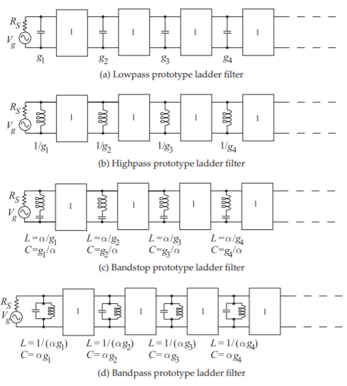
Figure \(\PageIndex{1}\): Ladder prototype filters.

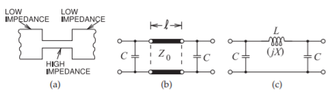
Figure \(\PageIndex{2}\): Inductive length of line with adjacent capacitive lines: (a) microstrip form; (b) lumped equivalent circuit; and (c) lumped-distributed equivalent circuit.

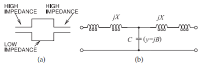
Figure \(\PageIndex{3}\): Capacitive length of line with adjacent inductive lines: (a) microstrip; and (b) lumped equivalent (the left-most and rightmost series inductors come from the high-impedance lines).

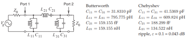
Figure \(\PageIndex{4}\): Lumped-element 3rd-order bandpass filters in a \(Z_{0} = 50\:\Omega\) system with center frequency \(f_{0} = 1\text{ GHz}\) and a \(3\text{ dB}\) bandwidth of \(10\%\).

so that the length of this predominantly inductive line is

\[\label{eq:2}\ell=\frac{\lambda_{g}}{2\pi}\sin^{-1}\left(\frac{\omega L}{Z_{0}}\right) \]

Previously it was shown that a short length of line having a relatively low characteristic impedance yields a capacitive element and this is shown, together with its equivalent circuit, in Figure \(\PageIndex{3}\). The predominating shunt capacitance is determined by first considering the susceptance

\[\label{eq:3}B=\frac{1}{Z_{0}}\sin\left(\frac{2\pi\ell}{\lambda_{g}}\right) \]

so that

\[\label{eq:4}\ell=\frac{\lambda_{g}}{2\pi}\sin^{-1}(\omega CZ_{0}) \]

Thus a cascade of low-impedance and high-impedance lines can realize (approximately) an \(LC\) ladder network.

It is tempting to take filters synthesized in lumped-element form and realize them in the above manner with transmission lines. The series element realization concept presented in this section could be extended using shorted and open stubs to better realize shunt elements. The problem with this approach is that the resulting filters are narrowband and the response outside the desired operating range is unpredictable. It is far better to employ the Richards’s transformation, considered in Section 2.12, which is a much broader bandwidth technique for realizing filters in distributed form.