4.11: 4.8 Radio Link Interference

Various excess delays on different paths causes intersymbol interference. High levels of intersymbol interference results in the failure to establish a communication link. Excess delay is a fundamental limitation with the 2G/GSM system and the only solution is to use very small cells in urban environments which have many significant signal paths. The 3G system employs a coding technique that enables the first few different paths to be resolved thus limiting the problem of ISI but not eliminating it. The 4G system, and 5G operates similarly, employs a long guard time, the cyclic prefix, to avoid ISI completely

4.8.1 Frequency Reuse Plan

Radio systems using the same channel are geographically spaced to control interference. In a cellular system, the coverage areas are arranged in cells represented by the hexagons in Figure \(\PageIndex{1}\). The actual shape of the cells is influenced by obstructions such as hills and buildings. In 1G and 2G cellular systems the cells are arranged in clusters such as the \(3-,\: 7-,\) and \(12\)-cell clusters shown, and the total number of channels available is divided among the cells in a cluster with the full set of frequency channels repeated in each cluster. (More about 3G–5G arrangements later.) The size of the clusters is the major component of what is called the frequency reuse plan. So a three-cell cluster has a spacing of approximately one cell diameter to the next cell using the same frequency channels. The signal level transmitted from the original cell will interfere with the signal in its corresponding cell in adjacent clusters. The level of interference is reduced with \(7\)-cell and then \(12\)-cell clusters. There is also background noise coming from cosmic sources as well as artificial sources, but in a cellular system, interference from other radios operating in the same system nearly always dominates.

The use of directional antennas at the base station increases the SIR. The interference pattern obtained using a trisector antenna (each segment of the antenna providing \(120^{\circ}\) of coverage) is shown in Figure \(\PageIndex{2}\). The trisector antenna can be arranged so that the transmit and receive antennas are

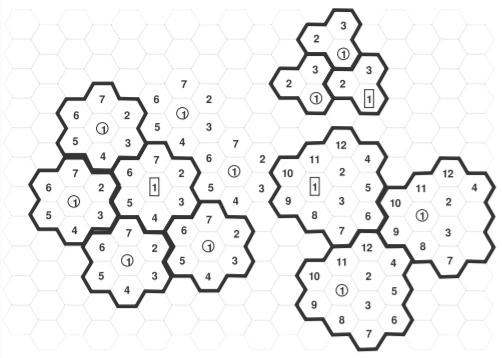
Figure \(\PageIndex{1}\): Cells arranged in clusters. Shown are \(3-\) cell clusters (top right), \(7-\) cell clusters (bottom left), and \(12-\)cell clusters (bottom right).

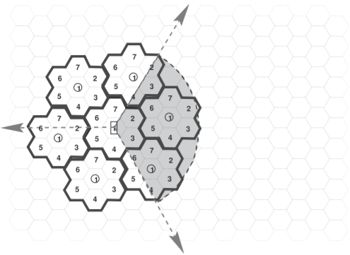
Figure \(\PageIndex{2}\): Cells in a cellular radio system with a trisector antenna, such as in Figure \(\PageIndex{3}\), showing the area of possible interference as a shaded region.

separated (see Figure \(\PageIndex{3}\)), and can also be arranged to tilt the coverage toward the ground (e.g., see the antenna in Figure 4.1.2(l)). It is also possible to use higher-order antenna sectoring and to have smaller cells (achieved possibly by relatively low-power transmissions) to provide higher levels of coverage at critical regions such as intersections of roads. These smaller cells are referred to as microcells or picocells.

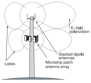
Figure \(\PageIndex{3}\): Base station with trisector stacked-dipole transmit and microstrip patch receive antennas.

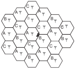
Figure \(\PageIndex{4}\): Three-cell cluster with mobile unit at the edge of cells \(\mathsf{A, B}\), and \(\mathsf{C}\).

Example \(\PageIndex{1}\): Cellular Interference

In a cellular system, a signal is intentionally transmitted from a base station nominally located in the center of a cell to a mobile unit in the same cell. However, nearby transmitters using the same channel cause interference. In Figure \(\PageIndex{4}\), a mobile unit is located at the edge of a cell and uses frequency channel A. Many nearby transmitters also operate using channel A and the six nearest transmitters can be considered as causing significant interference. Consider that the mobile unit is a distance \(r\) from its cell’s transmitter along the line connecting two channel A base stations, that the transmitters all operate at the same power level, and that the distance between base stations operating using channel A is \(3r\). This three-cell cluster operates in a suburban area and the power density drops off with distance \(d\) as \(1/d^{3}\) due to multipath effects. What is the SIR at the mobile unit?

Solution

There are seven close towers transmitting signals on the same channel. Call these \(A_{1}– A_{7}\) (\(M =\) mobile unit, \(A =\) transmitters). \(A_{1}\) is the desired signal and \(A_{2}–A_{7}\) are interferers. The distances from the transmitters to the mobile unit are \(d_{1}–d_{7}\), and the powers from the transmitters received at the mobile unit are \(P_{1}–P_{7}\).

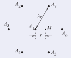
Figure \(\PageIndex{5}\)

Now \(\text{SIR}=\frac{P_{1}}{P_{2}+P_{3}+P_{4}+P_{5}+P_{6}+P_{7}}\)

This problem requires \(d_{2}–d_{7}\) to be determined.

Consider the diagram to the right with \(d_{1} = r\). Also, the distance from \(A_{2}\) to \(A_{7}\) is \(3r\). Now \(d_{3} = 3r + r = 4r,\: d_{6} = 3r − r = 2r\). So \(d_{2} = \left[(X + r)^{2} + Y^{2}\right]^{\frac{1}{2}} = (2.5^{2} + 2.6^{2})r = 3.607r = d_{4}\). (\(X = 3r\sin 30^{\circ} = 1.5r\) and \(Y = 3r\cos 30^{\circ} = 2.6r\).) Similarly \(d_{7} = d_{5} =\left[(1.5 − 1)^{2} + 2.6^{2}\right]^{\frac{1}{2}} = 2.648r\).

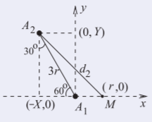
Figure \(\PageIndex{6}\)

\[\begin{array}{lll}{\frac{P_{2}}{P_{1}}=\frac{d_{1}}{d_{2}}=\frac{1}{3.607^{3}}=0.0213=\frac{P_{4}}{P_{1}}}&{\qquad}&{\frac{P_{3}}{P_{1}}=\frac{d_{1}}{d_{3}}=\frac{1}{4^{3}}=0.0156}\\{\frac{P_{7}}{P_{1}}=\frac{d_{1}}{d_{7}}=\frac{1}{2.648^{3}}=0.0539=\frac{P_{5}}{P_{1}}}&{\qquad}&{\frac{P_{6}}{P_{1}}=\frac{d_{1}}{d_{6}}=\frac{1}{2^{3}}=0.1250}\end{array}\nonumber \]

\[\text{SIR}=(0.0213 + 0.0156 + 0.0213 + 0.0539 + 0.1250 + 0.0539)^{−1} = 3.44 = 5.36\text{ dB}\nonumber \]

4.8.2 Summary

The clustering of cells as described above applies most directly to 1G and 2G cellular systems. The 3G system does not use clusters of cells but instead uses high frequency codes to separate users. There is a system awareness of managing interference but more complicated than the clustering arrangements. The 4G and 5G systems take frequency reuse algorithms to a whole new level performing global minimization of interference of wide areas. Still there is the basic concept that radios in adjacent cells operating on the same frequency channel can interfere with each other and careful attention must be given to frequency reuse.

The region of signal coverage by a basestation is greatly influenced by terrain and is not a neat hexagon. See for example the coverage map for a rural area shown in Figure 4.9.1(a). To ensure adequate coverage basestations must be placed on a terrain-aware grid and not a regular grid. A wasted expense in operating a cellular system would be installing more basestations than are needed for optimum coverage. Thus cellular service providers simulate coverage before installing basestations. A significant characteristic of urban coverage as shown in Figures 4.9.1(b and c) is the “urban canyon effect” whereby coverage is concentrated along roads with signals bouncing off buildings directing signal propagation down the roadway. Even areas close to a transmitter but behind buildings are shadowed while distant areas near roads can have good coverage. This effect is also known as the urban wave-guiding effect or wave-channeling effect. The signal blocking by buildings is shown in Figure 4.9.1(e) where it is seen that there is some diffraction over buildings but shadowing is severe after two or more diffraction events. The indoor environment also affects coverage as shown in Figure 4.9.1(d) for WiFi.