2.3: ADVANTAGES OF FEEDBACK

There is a frequent tendency on the part of the uninitiated to associate almost magical properties to feedback. Closer examination shows that many assumed benefits of feedback are illusory. The principal advantage is that feedback enables us to reduce the sensitivity of a system to changes in gain of certain elements. This reduction in sensitivity is obtained only in exchange for an increase in the magnitude of the gain of one or more of the elements in the system.

In some cases it is also possible to reduce the effects of disturbances applied to the system. We shall see that this moderation can always, at least conceptually, be accomplished without feedback, although the feedback approach is frequently a more practical solution. The limitations of this technique preclude reduction of such quantities as noise or drift at the input of an amplifier; thus feedback does not provide a method for detect­ing signals that cannot be detected by other means.

Feedback provides a convenient method of modifying the input and output impedance of amplifiers, although as with disturbance reduction, it is at least conceptually possible to obtain similar results without feedback.

Effect of Feedback on Changes in Open-Loop Gain

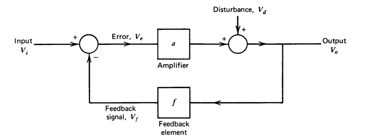
As mentioned above, the principal advantage of feedback systems com­pared with open-loop systems is that feedback provides a method for re­ducing the sensitivity of the system to changes in the gain of certain ele­ments. This advantage can be illustrated using the block diagram of Figure 2.2. If the disturbance is assumed to be zero, the closed-loop gain for the system is

\[\dfrac{V_o}{V_i} = \dfrac{a}{1 + af} \triangleq A \nonumber \]

(We will frequently use the capital letter \(A\) to denote closed-loop gain, while the lower-case a is normally reserved for a forward-path gain.)

The quantity af is the negative of the loop transmission for this system. The loop transmission is determined by setting all external inputs (and dis-­turbances) to zero, breaking the system at any point inside the loop, and determining the ratio of the signal returned by the system to an applied test input.(An example of this type of calculation is given in Section 2.4.1.) If the system is a negative feedback system, the loop transmission is negative. The negative sign on the summing point input that is included in the loop shown in Figure 2.2 indicates that the feedback is negative for this system if \(a\) and \(f\) have the same sign. Alternatively, the inversion necessary for negative feedback might be supplied by either the amplifier or the feed­back element.

Figure 2.2 Block diagram for the system of Figure 2.1.

Equation 2.2 shows that negative feedback lowers the magnitude of the gain of an amplifier since as \(f\) is increased from zero, the magnitude of the closed-loop gain decreases if \(a\) and \(f\) have this same sign. The result is general and can be used as a test for negative feedback.

It is also possible to design systems with positive feedback. Such systems are not as useful for our purposes and are not considered in detail.

The closed-loop gain expression shows that as the loop-transmission magnitude becomes large compared to unity, the closed-loop gain approac­hes the value \(1/f\). The significance of this relationship is as follows. The amplifier will normally include active elements whose characteristics vary as a function of age and operating conditions. This uncertainty may be unavoidable in that active elements are not available with the stability re­quired for a given application, or it may be introduced as a compromise in return for economic or other advantages.

Conversely, the feedback network normally attenuates signals, and thus can frequently be constructed using only passive components. Fortunately, passive components with stable, precisely known values are readily avail­able. If the magnitude of the loop transmission is sufficiently high, the closed-loop gain becomes dependent primarily on the characteristics of the feedback network.

This feature can be emphasized by calculating the fractional change in closed-loop gain \(d(V_o/V_i)/(V_o/V_i)\) caused by a given fractional change in amplifier forward-path gain \(da/a\), with the result

\[\dfrac{d(V_o/V_i)}{(V_o/V_i)} = \dfrac{da}{a} \left (\dfrac{1}{1 + af} \right ) \nonumber \]

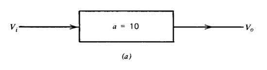
Equation 2.3 shows that changes in the magnitude of a can be attenuated to insignificant levels if \(af\) is sufficiently large. The quantity \(1 + af\) that relates changes in forward-path gain to changes in closed-loop gain is frequently called the desensitivity of a feedback system. Figure 2.3 illustrates this desensitization process by comparing two amplifier connections in­ tended to give an input-output gain of 10. Clearly the input-output gain is identically equal to a in Figure 2.3\(a\), and thus has the same fractional change in gain as does a. Equations 2.2 and 2.3 show that the closed-loop gain for the system of Figure 2.3\(b\) is approximately 9.9, and that the fractional change in closed-loop gain is less than 1%.of the fractional change in the forward- path gain of this system.

The desensitivity characteristic of the feedback process is obtained only in exchange for excess gain provided in the system. Returning to the ex­ample involving Figure 2.2, we see that the closed-loop gain for the system is \(a/(1 + af)\), while the forward-path gain provided by the amplifier is \(a\). The desensitivity is identically equal to the ratio of the forward-path gain to closed-loop gain. Feedback connections are unique in their ability to automatically trade excess gain for desensitivity.

It is important to underline the fact that changes in the gain of the feed­back element have direct influence on the closed-loop gain of the system, and we therefore conclude that it is necessary to observe or measure the output variable of a feedback system accurately in order to realize the advantages of feedback.

Figure 2.3 Amplifier connections for a gain of ten. (a) Open loop. (b) Closed loop.

Effect of Feedback on Nonlinearities

Because feedback reduces the sensitivity of a system to changes in open-loop gain, it can often moderate the effects of nonlinearities. Figure 2.4 illustrates this process. The forward path in this connection consists of an amplifier with a gain of 1000 followed by a nonlinear element that might be an idealized representation of the transfer characteristics of a power output stage. The transfer characteristics of the nonlinear element show these four distinct regions:

1. A deadzone, where the output remains zero until the input magnitude exceeds 1 volt. This region models the crossover distortion associated with many types of power amplifiers.
2. A linear region, where the incremental gain of the element is one.
3. A region of soft limiting, where the incremental gain of the element is lowered to 0.1.
4. A region of hard limiting or saturation where the incremental gain of the element is zero.

The performance of the system can be determined by recognizing that, since the nonlinear element is piecewise linear, all transfer relationships must be piecewise linear. The values of all the variables at a breakpoint can be found by an iterative process. Assume, for example, that the variables associated with the nonlinear element are such that this element is at its breakpoint connecting a slope of zero to a slope of +1. This condition only occurs for \(v_A = 1\) and \(v_B = 0\). If \(v_B = v_O = 0\), the signal \(v_F\) must be zero, since \(v_F = 0.1 v_O\). Similarly, with \(v_A = 1, v_E = 10^{-3} v_A = 10^{-3}\). Since the relationships at the summing point imply \(v_E = v_I - v_F\), or \(v_I = v_E + v_F\), \(v_I\) must equal \(10^{-3}\). The values of variables at all other breakpoints can be found by similar reasoning. Results are summarized in Table 2.1.

Table 2.1 Values of Variables at Breakpoints for System of Figure 2.4

\(v_I\)	\(v_E = v_I - v_F\)	\(v_A = 10^3 v_E\)	\(v_B = v_O\)	\(v_F = 0.1 v_O\)
<-0.258	\(v_I + 0.250\)	\(10^3 v_I + 250\)	-2.5	-0.25
-0.258	-0.008	-8	-2.5	-0.25
-0.203	-0.003	-3	-2	-0.2
\(-10^{-3}\)	\(-10^{-3}\)	-1	0	0
\(10^{-3}\)	\(10^{-3}\)	1	0	0
0.203	0.003	3	2	0.2
0.258	0.008	8	2.5	0.25
>0.258	\(v_I - 0.250\)	\(10^3 v_I - 250\)	2.5	0.25

The input-output transfer relationship for the system shown in Figure 2.4\(c\) is generated from values included in Table 2.1. The transfer relationship can also be found by using the incremental forward gain, or 1000 times the incremental gain of the nonlinear element, as the value for \(a\) in Equation 2.2. If the magnitude of signal \(v_A\) is less than 1 volt, a is zero, and the incremental closed-loop gain of the system is also zero. If \(v_A\) is between 1 and 3 volts, a is \(10^3\), so the incremental closed-loop gain is 9.9. Similarly, the incre­ mental closed-loop gain is 9.1 for \(3 < v_A < 8\).

Note from Figure 2.4\(c\) that feedback dramatically reduces the width of the deadzone and the change in gain as the output stage soft limits. Once the amplifier saturates, the incremental loop transmission becomes zero, and as a result feedback cannot improve performance in this region.

Figure 2.4 The effects of feedback on a nonlinearity. (a) System. (b) Transfer characteristics of the nonlinear element. (c) System transfer characteristics (closed loop). (Not to scale.) (d) Waveforms for \(v_I (t)\) a unit ramp. (Not to scale.)

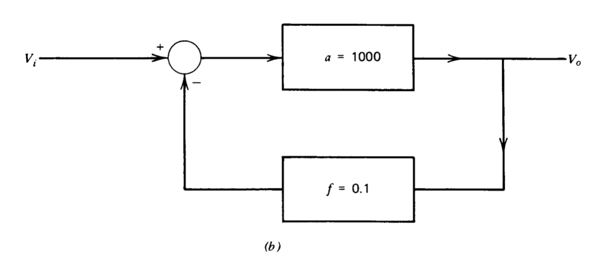
Figure 2.4\(d\) provides insight into the operation of the circuit by compar­ing the output of the system and the voltage \(v_A\) for a unit ramp input. The output remains a good approximation to the input until saturation is reached. The signal into the nonlinear element is "predistorted" by feedback in such a way as to force the output from this element to be nearly linear.

The technique of employing feedback to reduce the effects of nonlinear elements on system performance is a powerful and widely used method that evolves directly from the desensitivity to gain changes provided by feedback. In some applications, feedback is used to counteract the un­avoidable nonlinearities associated with active elements. In other applica­tions, feedback is used to maintain performance when nonlinearities result from economic compromises. Consider the power amplifier that provided the motivation for the previous example. The designs for linear power- handling stages are complex and expensive because compensation for the base-to-emitter voltages of the transistors and variations of gain with operating point must be included. Economic advantages normally result if linearity of the power-handling stage is reduced and low-power voltage-gain stages (possibly in the form of an operational amplifier) are added prior to the output stage so that feedback can be used to restore system linearity.

While this section has highlighted the use of feedback to reduce the effects of nonlinearities associated with the forward-gain element of a sys­tem, feedback can also be used to produce nonlinearities with well-con­trolled characteristics. If the feedback element in a system with large loop transmission is nonlinear, the output of the system becomes approximately \(v_O = f^{-1} (v_I)\). Here \(f^{-1}\) is the inverse of the feedback-element transfer rela­tionship, in the sense that \(f^{-1} [f(V)] = V\). For example, transistors or diodes with exponential characteristics can be used as feedback elements around an operational amplifier to provide a logarithmic closed-loop transfer relationship.

Disturbances in Feedback Systems

Feedback provides a method for reducing the sensitivity of a system to certain kinds of disturbances. This advantage is illustrated in Figure 2.5. Three different sources of disturbances are applied to this system. The disturbance \(V_{d1}\) enters the system at the same point as the system input, and might represent the noise associated with the input stage of an amplifier. Disturbance \(V_{d2}\) enters the system at an intermediate point, and might represent a disturbance from the hum associated with the poorly filtered voltage often used to power an amplifier output stage. Disturbance \(V_{d3}\) enters at the amplifier output and might represent changing load characteristics.

Figure 2.5 Feedback system illustrating effects of disturbances.

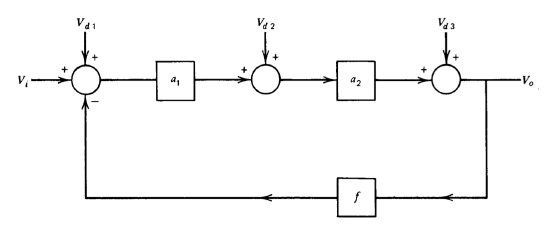
The reader should convince himself that the block diagram of Figure 2.5 implies that the output voltage is related to input and disturbances as

\[V_o = \dfrac{a_1 a_2 [(V_i + V_{d1}) + (V_{d2}/a_1) + (V_{d3}/a_1 a_2)]}{1 + a_1 a_2 f} \nonumber \]

Equation 2.4 shows that the disturbance \(V_{d1}\) is not attenuated relative to the input signal. This result is expected since \(V_i\) and \(V_{d1}\) enter the system at the same point, and reflects the fact that feedback cannot improve quan­tities such as the noise figure of an amplifier. The disturbances that enter the amplifier at other points are attenuated relative to the input signal by amounts equal to the forward-path gains between the input and the points where the disturbances are applied.

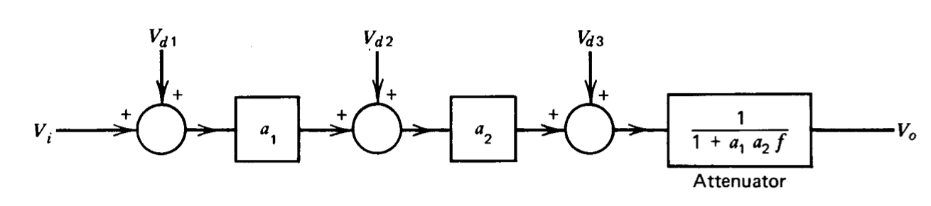
It is important to emphasize that the forward-path gain preceding the disturbance, rather than the feedback, results in the relative attenuation of the disturbance. This feature is illustrated in Figure 2.6. This open-loop system, which follows the forward path of Figure 2.5 with an attenuator, yields the same output as the feedback system of Figure 2.5. The feedback system is nearly always the more practical approach, since the open-loop system requires large signals, with attendant problems of saturation and power dissipation, at the input to the attenuator. Conversely, the feedback realiza­tion constrains system variables to more realistic levels.

Summary

This section has shown how feedback can be used to desensitize a system to changes in component values or to externally applied disturbances. This desensitivity can only be obtained in return for increases in the gains of various components of the system. There are numerous situations where this type of trade is advantageous. For example, it may be possible to replace a costly, linear output stage in a high-fidelity audio amplifier with a cheaper unit and compensate for this change by adding an inexpensive stage of low-level amplification.

Figure 2.6 Open-loop system illustrating effects of disturbances.

The input and output impedances of amplifiers are also modified by feed­back. For example, if the output variable that is fed back is a voltage, the feedback tends to stabilize the value of this voltage and reduce its depend­ence on disturbing load currents, implying that the feedback results in lower output impedance. Alternatively, if the information fed back is proportional to output current, the feedback raises the output impedance. Similarly, feedback can limit input voltage or current applied to an ampli­fier, resulting in low or high input impedance respectively. A quantitative discussion of this effect is reserved for Section 2.5.

A word of caution is in order to moderate the impression that perform­ance improvements always accompany increases in loop-transmission magnitude. Unfortunately, the loop transmission of a system cannot be increased without limit, since sufficiently high gain invariably causes a sys­tem to become unstable. A stable system is defined as one for which a bounded output is produced in response to a bounded input. Conversely, an unstable system exhibits runaway or oscillatory behavior in response to a bounded input. Instability occurs in high-gain systems because small errors give rise to large corrective action. The propagation of signals around the loop is delayed by the dynamics of the elements in the loop, and as a consequence high-gain systems tend to overcorrect. When this overcorrec­tion produces an error larger than the initiating error, the.system is unstable.

This important aspect of the feedback problem did not appear in this section since the dynamics associated with various elements have been ig­nored. The problem of stability will be investigated in detail in Chapter 4.