
3.5: RELATIONSHIPS BETWEEN TRANSIENT RESPONSE AND FREQUENCY RESPONSE
- Page ID
- 60844

\( \newcommand{\vecs}[1]{\overset { \scriptstyle \rightharpoonup} {\mathbf{#1}} } \)
\( \newcommand{\vecd}[1]{\overset{-\!-\!\rightharpoonup}{\vphantom{a}\smash {#1}}} \)
\( \newcommand{\id}{\mathrm{id}}\) \( \newcommand{\Span}{\mathrm{span}}\)
( \newcommand{\kernel}{\mathrm{null}\,}\) \( \newcommand{\range}{\mathrm{range}\,}\)
\( \newcommand{\RealPart}{\mathrm{Re}}\) \( \newcommand{\ImaginaryPart}{\mathrm{Im}}\)
\( \newcommand{\Argument}{\mathrm{Arg}}\) \( \newcommand{\norm}[1]{\| #1 \|}\)
\( \newcommand{\inner}[2]{\langle #1, #2 \rangle}\)
\( \newcommand{\Span}{\mathrm{span}}\)
\( \newcommand{\id}{\mathrm{id}}\)
\( \newcommand{\Span}{\mathrm{span}}\)
\( \newcommand{\kernel}{\mathrm{null}\,}\)
\( \newcommand{\range}{\mathrm{range}\,}\)
\( \newcommand{\RealPart}{\mathrm{Re}}\)
\( \newcommand{\ImaginaryPart}{\mathrm{Im}}\)
\( \newcommand{\Argument}{\mathrm{Arg}}\)
\( \newcommand{\norm}[1]{\| #1 \|}\)
\( \newcommand{\inner}[2]{\langle #1, #2 \rangle}\)
\( \newcommand{\Span}{\mathrm{span}}\) \( \newcommand{\AA}{\unicode[.8,0]{x212B}}\)
\( \newcommand{\vectorA}[1]{\vec{#1}} % arrow\)
\( \newcommand{\vectorAt}[1]{\vec{\text{#1}}} % arrow\)
\( \newcommand{\vectorB}[1]{\overset { \scriptstyle \rightharpoonup} {\mathbf{#1}} } \)
\( \newcommand{\vectorC}[1]{\textbf{#1}} \)
\( \newcommand{\vectorD}[1]{\overrightarrow{#1}} \)
\( \newcommand{\vectorDt}[1]{\overrightarrow{\text{#1}}} \)
\( \newcommand{\vectE}[1]{\overset{-\!-\!\rightharpoonup}{\vphantom{a}\smash{\mathbf {#1}}}} \)
\( \newcommand{\vecs}[1]{\overset { \scriptstyle \rightharpoonup} {\mathbf{#1}} } \)
\( \newcommand{\vecd}[1]{\overset{-\!-\!\rightharpoonup}{\vphantom{a}\smash {#1}}} \)
\(\newcommand{\avec}{\mathbf a}\) \(\newcommand{\bvec}{\mathbf b}\) \(\newcommand{\cvec}{\mathbf c}\) \(\newcommand{\dvec}{\mathbf d}\) \(\newcommand{\dtil}{\widetilde{\mathbf d}}\) \(\newcommand{\evec}{\mathbf e}\) \(\newcommand{\fvec}{\mathbf f}\) \(\newcommand{\nvec}{\mathbf n}\) \(\newcommand{\pvec}{\mathbf p}\) \(\newcommand{\qvec}{\mathbf q}\) \(\newcommand{\svec}{\mathbf s}\) \(\newcommand{\tvec}{\mathbf t}\) \(\newcommand{\uvec}{\mathbf u}\) \(\newcommand{\vvec}{\mathbf v}\) \(\newcommand{\wvec}{\mathbf w}\) \(\newcommand{\xvec}{\mathbf x}\) \(\newcommand{\yvec}{\mathbf y}\) \(\newcommand{\zvec}{\mathbf z}\) \(\newcommand{\rvec}{\mathbf r}\) \(\newcommand{\mvec}{\mathbf m}\) \(\newcommand{\zerovec}{\mathbf 0}\) \(\newcommand{\onevec}{\mathbf 1}\) \(\newcommand{\real}{\mathbb R}\) \(\newcommand{\twovec}[2]{\left[\begin{array}{r}#1 \\ #2 \end{array}\right]}\) \(\newcommand{\ctwovec}[2]{\left[\begin{array}{c}#1 \\ #2 \end{array}\right]}\) \(\newcommand{\threevec}[3]{\left[\begin{array}{r}#1 \\ #2 \\ #3 \end{array}\right]}\) \(\newcommand{\cthreevec}[3]{\left[\begin{array}{c}#1 \\ #2 \\ #3 \end{array}\right]}\) \(\newcommand{\fourvec}[4]{\left[\begin{array}{r}#1 \\ #2 \\ #3 \\ #4 \end{array}\right]}\) \(\newcommand{\cfourvec}[4]{\left[\begin{array}{c}#1 \\ #2 \\ #3 \\ #4 \end{array}\right]}\) \(\newcommand{\fivevec}[5]{\left[\begin{array}{r}#1 \\ #2 \\ #3 \\ #4 \\ #5 \\ \end{array}\right]}\) \(\newcommand{\cfivevec}[5]{\left[\begin{array}{c}#1 \\ #2 \\ #3 \\ #4 \\ #5 \\ \end{array}\right]}\) \(\newcommand{\mattwo}[4]{\left[\begin{array}{rr}#1 \amp #2 \\ #3 \amp #4 \\ \end{array}\right]}\) \(\newcommand{\laspan}[1]{\text{Span}\{#1\}}\) \(\newcommand{\bcal}{\cal B}\) \(\newcommand{\ccal}{\cal C}\) \(\newcommand{\scal}{\cal S}\) \(\newcommand{\wcal}{\cal W}\) \(\newcommand{\ecal}{\cal E}\) \(\newcommand{\coords}[2]{\left\{#1\right\}_{#2}}\) \(\newcommand{\gray}[1]{\color{gray}{#1}}\) \(\newcommand{\lgray}[1]{\color{lightgray}{#1}}\) \(\newcommand{\rank}{\operatorname{rank}}\) \(\newcommand{\row}{\text{Row}}\) \(\newcommand{\col}{\text{Col}}\) \(\renewcommand{\row}{\text{Row}}\) \(\newcommand{\nul}{\text{Nul}}\) \(\newcommand{\var}{\text{Var}}\) \(\newcommand{\corr}{\text{corr}}\) \(\newcommand{\len}[1]{\left|#1\right|}\) \(\newcommand{\bbar}{\overline{\bvec}}\) \(\newcommand{\bhat}{\widehat{\bvec}}\) \(\newcommand{\bperp}{\bvec^\perp}\) \(\newcommand{\xhat}{\widehat{\xvec}}\) \(\newcommand{\vhat}{\widehat{\vvec}}\) \(\newcommand{\uhat}{\widehat{\uvec}}\) \(\newcommand{\what}{\widehat{\wvec}}\) \(\newcommand{\Sighat}{\widehat{\Sigma}}\) \(\newcommand{\lt}{<}\) \(\newcommand{\gt}{>}\) \(\newcommand{\amp}{&}\) \(\definecolor{fillinmathshade}{gray}{0.9}\)It is clear that either the impulse response (or the response to any other transient input) of a linear system or its frequency response completely characterize the system. In many cases experimental measurements on a closed-loop system are most easily made by applying a transient input. We may, however, be interested in certain aspects of the frequency response of the system such as its bandwidth defined as the frequency where its gain drops to 0.707 of the midfrequency value.
Since either the transient response or the frequency response completely characterize the system, it should be possible to determine performance in one domain from measurements made in the other. Unfortunately, since the measured transient response does not provide an equation for this
response, Laplace techniques cannot be used directly unless the time response is first approximated analytically as a function of time. This section lists several approximate relationships between transient response and frequency response that can be used to estimate one performance measure from the other. The approximations are based on the properties of first- and second-order systems.
It is assumed that the feedback path for the system under study is frequency independent and has a magnitude of unity. A system with a fre quency-independent feedback path fo can be manipulated as shown in Figure 3.16 to yield a scaled, unity-feedback system. The approximations given are valid for the transfer function \(V_a/V_i\), and \(V_o\) can be determined by scaling values for \(V_a\) by \(1/f_o\).
It is also assumed that the magnitude of the d-c loop transmission is very large so that the closed-loop gain is nearly one at d-c. It is further assumed that the singularity closest to the origin in the s plane is either a pole or a complex pair of poles, and that the number of poles of the function exceeds
the number of zeros. If these assumptions are satisfied, many practical systems have time domain-frequency domain relationships similar to those of first- or second-order systems.
The parameters we shall use to describe the transient response and the frequency response of a system include the following.
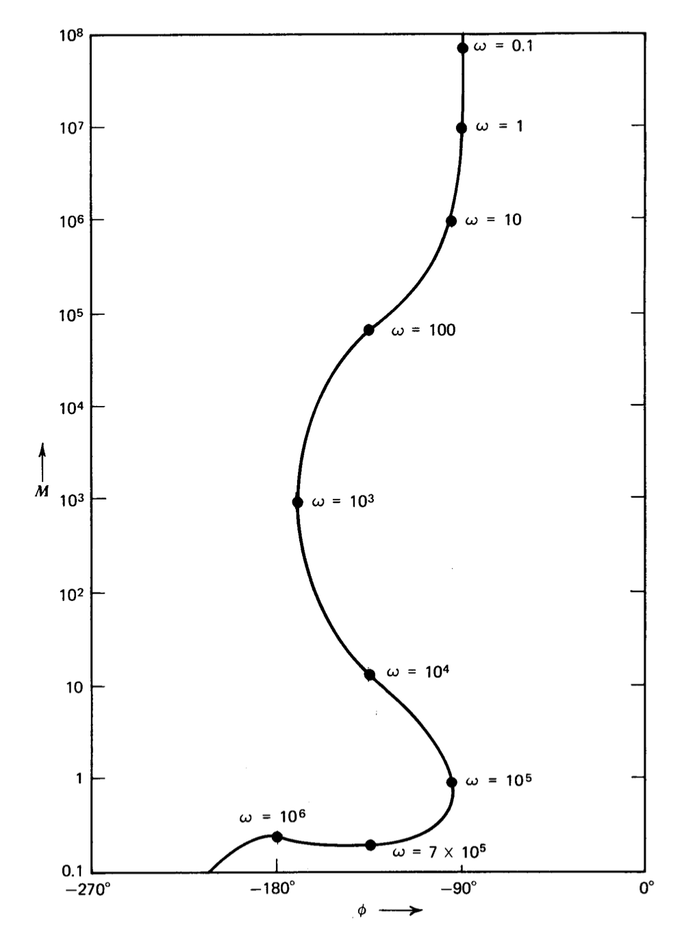
Figure 3.15 Gain phase plot of \(\dfrac{10^7 (10^{-4} s + 1)}{s(0.1s + 1)(s^2/10^{12} + 2 (0.2) s/10^6 + 1)}\).
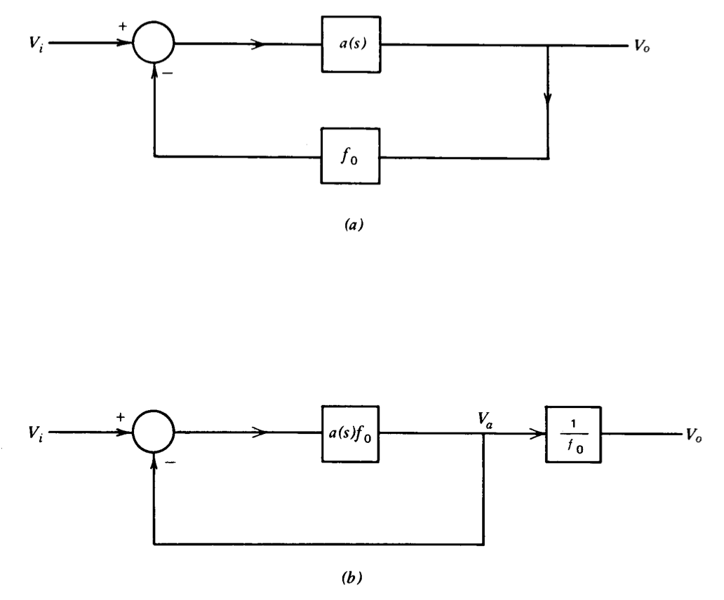
Figure 3.16 System topology for approximate relationships. (\(a\)) System with frequency-independent feedback path. (\(b\)) System represented in scaled, unity-feedback form.
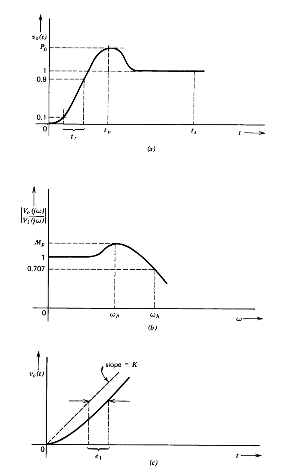
(a) Rise time \(t_r\). The time required for the step response to go from 10 to 90 % of final value.
(b) The maximum value of the step response \(P_0\).
(c) The time at which \(P_0\) occurs \(t_p\).
(d) Settling time \(t_s\). The time after which the system step response remains within 2% of final value.
(e) The error coefficient ei. (See Section 3.6.) This coefficient is equal to the time delay between the output and the input when the system has reached steady-state conditions with a ramp as its input.
(f) The bandwidth in radians per second \(w_h\) or hertz \(f_h\) (\(f_h = \omega_h/2\pi\)). The frequency at which the response of the system is 0.707 of its low-frequency value.
(g) The maximum magnitude of the frequency response \(M_p\).
(h) The frequency at which \(M_p\) occurs \(\omega_p\).
These definitions are illustrated in Figure 3.17.
For a first-order system with \(V_o (s)/V_i (s) = 1/(\tau s + 1)\), the relationships are
\[t_r = 2.2 \tau = \dfrac{2.2}{\omega_h} = \dfrac{0.35}{f_h}\label{eq3.5.1} \]
\[P_0 = M_p = 1 \nonumber \]
\[t_p = \infty \nonumber \]
\[t_s = 4\tau \nonumber \]
\[e_1 = \tau \nonumber \]
\[\omega_p = 0 \nonumber \]
For a second-order system with \(V_o (s)/V_i (s) = 1/(s^2/\omega_n^2 + 2 \zeta s/\omega_n + 1)\) and \(\theta \triangleq \cos^{-1} \zeta\) (see Figure3.7) the relationships are
\[t_r \simeq \dfrac{2.2}{\omega_h} = \dfrac{0.35}{f_h}\label{eq3.5.7} \]
\[P_0 = 1 + \exp \dfrac{-\pi \zeta}{\sqrt{1 - \zeta^2}} = 1 + e^{-\pi/\tan \theta}. \nonumber \]
\[t_p = \dfrac{\pi}{\omega_n \sqrt{1 - \zeta^2}} = \dfrac{\pi}{\omega_n \sin \theta} \nonumber \]
\[t_s \simeq \dfrac{4}{\zeta \omega_n} = \dfrac{4}{\omega_n \cos \theta} \nonumber \]
\[e_1 = \dfrac{2 \zeta}{\omega_n} = \dfrac{2\cos \theta}{\omega_n} \nonumber \]
\[M_p = \dfrac{1}{2\zeta \sqrt{1 - \zeta^2}} = \dfrac{1}{\sin 2 \theta} \ \ \zeta < 0.707, \theta > 45^{\circ} \nonumber \]
\[\omega_p = \omega_n \sqrt{1 - 2\zeta^2} = \omega_n \sqrt{-\cos 2\theta} \ \ \zeta < 0.707, \theta > 45^{\circ} \nonumber \]
\[\omega_h = \omega_n (1 - 2 \zeta^2 + \sqrt{2 - 4\zeta^2 + 4\zeta^4})^{1/2} \nonumber \]
If a system step response or frequency response is similar to that of an approximating system (see Figs. 3.6, 3.8, 3.11, and 3.12) measurements of \(t_r\), \(P_0\), and \(t_p\) permit estimation of \(\omega_h\), \(\omega_p\), and \(M_p\) or vice versa. The steady-state error in response to a unit ramp can be estimated from either set of measurements.
One final comment concerning the quality of the relationship between 0.707 bandwidth and 10 to 90% step risetime (Equations \(\ref{eq3.5.1}\) and \(\ref{eq3.5.7}\)) is in order. For virtually any system that satisfies the original assumptions, independent of the order or relative stability of the system, the product \(t_rf_h\) is within a few percent of 0.35. This relationship is so accurate that it really isn't worth measuring \(f_h\) if the step response can be more easily determined.