12.4: ACTIVE FILTERS

There are numerous applications that require the realization of a particu­lar transfer function. One of the many limitations of the design of filter networks using only passive components is that inductors are required to obtain complex pole locations. This restriction is removed if active elements are included in the designs, and the resultant active filters permit the realiza­tion of complex poles using only resistors and capacitors in addition to the active elements. Further advantages of active-filter synthesis include the possibility of a wide range of relative input and output impedances, and the use of smaller, less expensive reactive components than is normally possible with passive designs.

There is a fair amount of present research devoted toward improving techniques for active-filter synthesis, and the probability is that better de­signs, particularly with respect to sensitivity (the dependence of the transfer function on variations in parameter values), will evolve. This section de­scribes two presently popular topologies that can be used to realize active filters.

Sallen and Key Circuit

R. P. Sallen and E. L. Key, "A Practical Method of Designing RC Active Filters," Insti­tute of Radio Engineers, Transactions on Circuit Theory, March, 1955, pp. 74-85.

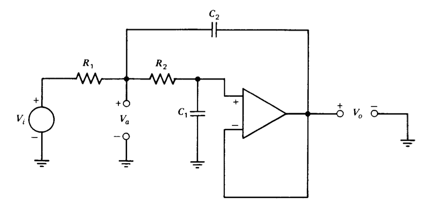
Figure 12.22 Second-order low-pass active filter.

Figure 12.22 shows an active-filter circuit that uses a unity-gain-con­nected operational amplifier. Node equations for the circuit are easily written by noting that the voltage at the noninverting input of the amplifier is equal to the output voltage and are

\[\begin{array} {rcl} {G_1 V_i} & = & {(G_1 + G_2 + C_2s)V_a - (G_2 + C_2s)V_o} \\ {0} & = & {-G_2 V_a + (G_2 + C_1 s)V_o} \end{array} \nonumber \]

Solving for the transfer function yields

\[\dfrac{V_o (s)}{V_i (s)} = \dfrac{1}{R_1 R_2 C_1 C_2 s^2 + (R_1 + R_2) C_1 s + 1} \nonumber \]

This equation represents a second-order transfer function with standard- form parameters

\[\omega_n = \dfrac{1}{\sqrt{R_1 R_2 C_1 C_2}} \nonumber \]

and

\[\zeta = \dfrac{R_1 + R_2}{2 \sqrt{R_1R_2}} \sqrt{\dfrac{C_1}{C_2}} \nonumber \]

Since only two quantities are required to characterize the second-order filter, the four degrees of freedom represented by the four passive-com­ponent values are redundant. Part of this redundancy is frequently elimi­nated by choosing \(R_1 = R_2 = R\). In this case, the standard-form param­eters become

\[\omega_n = \dfrac{1}{R\sqrt{C_1 C_2}} \nonumber \]

and

\[\zeta = \sqrt{\dfrac{C_1}{C_2}} \nonumber \]

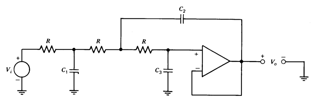
Figure 12.23 Third-order low-pass active filter.

The addition of another section to the second-order low-pass active filter as shown in Figure 12.23 allows the synthesis of a third-order transfer function with a single amplifier. If equal-value resistors are used as shown, the transfer function is

\[\dfrac{V_o(s)}{V_i (s)} = \dfrac{1}{C_1 C_2 C_3 R^3 s^3 + 2(C_1 C_3 + C_2 C_3) R^2 s^2 + (C_1 + 3C_3) Rs + 1} \nonumber \]

An \(n\)th-order low-pass filter is often designed by combining \(n/2\) second-order sections in the case of n even, or one third-order section with \(n/2 - 3/2\) second-order sections when \(n\) is odd. Tables(Farouk Al-Nasser, "Tables Speed Design of Low-Pass Active Filters," EDN, March 15, 1971, pp. 23-32. ) that simplify element-value selection are available for filters up to the tenth order with a number of different pole patterns.

Figure 12.24 Second-order high-pass active filter.

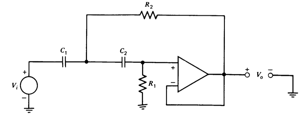
Interchanging resistors and capacitors as shown in Figure 12.24 changes the second-order low-pass filter to a high-pass filter. The transfer function for this configuration is

\[\dfrac{V_o (s)}{V_i (s)} = \dfrac{R_1 R_2 C_1 C_2 s^2}{R_1 R_2 C_1 C_2 s^2 + R_2 (C_1 + C_2) s + 1}\label{eq12.4.8} \]

If, in a development analogous to that used for the low-pass filter, we choose \(C_1 = C_2 = C\), Equation \(\ref{eq12.4.8}\) reduces to

\[\dfrac{V_o (s)}{V_i (s)} = \dfrac{s^2/\omega_n^2}{(s^2/\omega_n^2) + (2\zeta s/\omega_n) + 1} \nonumber \]

where

\[\omega_n = \dfrac{1}{C\sqrt{R_1 R_2}}\nonumber \]

and

\[\zeta = \sqrt{\dfrac{R_2}{R_1}}\nonumber \]

The Sallen and Key circuit can be designed with an amplifier gain other than unity (see Problem P12.8). This modification allows greater flexibility, since the low- or high-frequency gain of the circuit can be made other than one. However, the damping ratio of transfer functions realized in this way is dependent on the values of resistors that set the closed-loop amplifier gain; thus poles may be somewhat less reliably located. A further advantage of the unity-gain version is that it may be constructed using the LM 110 inte­grated circuit (see Section 10.4.4). The bandwidth of this amplifier far exceeds that of most general-purpose integrated-circuit units, and corner frequencies in the low megahertz range can be obtained using it.

General Synthesis Procedure

The Sallen and Key configuration, together with many other active- filter topologies, allows-complete freedom in the choice of pole location, but does not permit arbitrary placement of transfer-function zeros. The application of the analog-computation concepts described in Section 12.3.1 allows the synthesis of any realizable transfer function that is expressable as a ratio of polynomials in s, provided that the number of poles is equal to or greater than the number of zeros in the transfer function.

Consider the transfer function

\[\dfrac{V_o (s)}{V_i (s)} = \dfrac{b_n s^n + b_{n - 1} s^{n - 1} + \cdots + b_1 s + b_0}{a_n s^n + a_{n - 1} s^{n - 1} + \cdots + a_1 s + a_0}\label{eq12.4.10} \]

The first step is to introduce an intermediate variable \(V_a (s)\) such that \(V_a(s)/ V_i(s)\) contains only the poles of the transfer function, or

\[\dfrac{V_o (s)}{V_i (s)} = \dfrac{1}{a_n s^n + a_{n - 1} s^{n - 1} + \cdots + a_1 s + a_0} \nonumber \]

Proceeding in a way exactly parallel to the time-domain development of Section 12.3.1, we write

\[s^n V_a (s) = -\dfrac{a_{n - 1}}{a_n} s^{n -1} V_a (s) - \cdots - \dfrac{a_1}{a_n} s V_a (s) - \dfrac{a_0}{a_n} V_a (s) + \dfrac{V_i (s)}{a_n} \label{eq12.4.12} \]

Figure 12.25 Block diagram representation of transfer function that contains only poles.

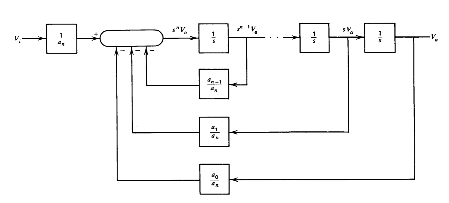
The block-diagram representation of Equation \(\ref{eq12.4.12}\) is shown in Figure 12.25. This block diagram can be readily implemented using summers and inte­ grators. In order to complete the synthesis of our transfer function (Equation \(\ref{eq12.4.10}\)) we recognize that

\[V_o (s) = V_a (s) (b_n s^n + b_{n - 1} s^{n - 1} + \cdots + b_1 s + b_0)\label{eq12.4.13} \]

The essential feature of Equation \(\ref{eq12.4.13}\) is that it indicates \(V_o(s)\) is a linear com­bination of \(V_a(s)\) and its first \(n\) derivatives. Since all of the necessary vari­ables appear in the block diagram, \(V_o (s)\) can be generated by simply scaling and summing these variables, without the need for differentiation.

This synthesis procedure is illustrated for an approximation to a pure time delay known as the Pade approximate. The time delay has a transfer function \(e^{-s \tau}\), where \(\tau\) is the length of the delay. The magnitude of this trans­fer function is one at all frequencies, while its negative phase shift is linearly proportional to frequency. The time delay has an essential singularity at the origin, and thus cannot be exactly represented as a ratio of polynomials in \(s\).

The Taylor's series expansion of \(e^{-s \tau}\) is

\[e^{-s\tau} = 1 - s \tau + \dfrac{s^2 \tau^2}{2!} - \cdots + \cdots + (-1)^m \dfrac{s^m \tau^m}{m!} + \cdots \nonumber \]

The Pade approximates locate an equal number of poles and zeros so as to agree with the maximum possible number of terms of the Taylor's series expansion. This approximation always leads to an all-pass network that has right-half-plane zeros and left-half-plane poles located symmetrically with respect to the imaginary axis. This type of singularity pattern results in a frequency-independent magnitude for the transfer function.

Since we can always frequency or time scale at a later point, we consider a unit time delay \(e^{-s}\) to simplify the development. The first-order Pade approximate to this function is

\[P_1 (s) = \dfrac{1 - (s/2)}{1 + (s/2)} = 1 - s + \dfrac{s^2}{2} - \dfrac{s^3}{4} + \cdots - \cdots + \nonumber \]

The expansion for \(e^{-s}\) is

\[e^{-s} = 1 - s + \dfrac{s^2}{2} - \dfrac{s^3}{6} + \dfrac{s^4}{24} - \dfrac{s^5}{120} + \dfrac{s^6}{720} - \cdots + \nonumber \]

The first-order approximation matches the first two coefficients of \(s\) of the complete expansion, and is in reasonable agreement with the third coefficient. This match is all that can be expected, since only two degrees of freedom (the location of the pole and the location of the zero) are available for the first-order approximation. The second-order Pade approximate to a one-second time delay is

\[P_2 (s) = \dfrac{1 - (s/2) + (s^2/12)}{1 + (s/2) + (s^2/12)} = 1 - s + \dfrac{s^2}{2} - \dfrac{s^2}{2} - \dfrac{s^3}{6} + \dfrac{s^4}{24} - \dfrac{s^5}{144} + \cdots - \cdots +\label{eq12.4.17} \]

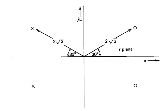
Figure 12.26 Singularity locations for second-order Pade approximate to one-second time delay.

As expected, the first four time-delay coefficients of \(s\) are matched by the approximation. The \(s\)-plane plot for \(P_2(s)\) is shown in Figure 12.26. Simple vector manipulations confirm the fact that the magnitude of this function is one at all frequencies.

The phase shift of the approximating function is (from Equation \(\ref{eq12.4.17}\))

\[\measuredangle P_2 (j \omega) = 2\measuredangle \left [1 - \dfrac{j \omega}{2} + \dfrac{(j \omega)^2}{12} \right ] = -2 \tan^{-1} \left \{\dfrac{\omega}{2[1 - (\omega^2/12)]} \right \} \nonumber \]

Figure 12.27 Comparison of time delay and Pad6 approximate phase characteristics.

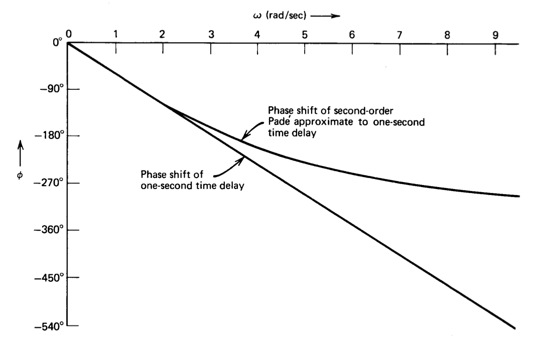
This function is compared with an angle of \(-57.3^{\circ} \omega\) (the value for a one-second time delay) in Figure 12.27. We note excellent agreement to frequencies of approximately 2 radians per second implying that the approximation represents the actual function well for sinusoidal excitation to this fre­quency, with increasing discrepancy at higher frequencies. The error re­flects the fact that the maximum negative phase shift of the Pade approxi­mate is \(360^{\circ}\), while the time delay provides unlimited negative phase shift at sufficiently high frequency.

Synthesis is initiated by defining an intermediate variable \(V_a (s)\) in accord­ance with Equations \(\ref{eq12.4.11}\) and \(\ref{eq12.4.12}\), or

\[\dfrac{V_a(s)}{V_i (s)} = \dfrac{1}{(s^2/12) + (s/2) + 1} \nonumber \]

and

\[s^2 V_a (s) = -6s V_o (s) - 12V_a (s) + 12 V_i (s) \nonumber \]

The output voltage is

\[V_o (s) = \dfrac{s^2}{12} V_a (s) - \dfrac{s}{2} V_a (s) + V_a (s) \nonumber \]

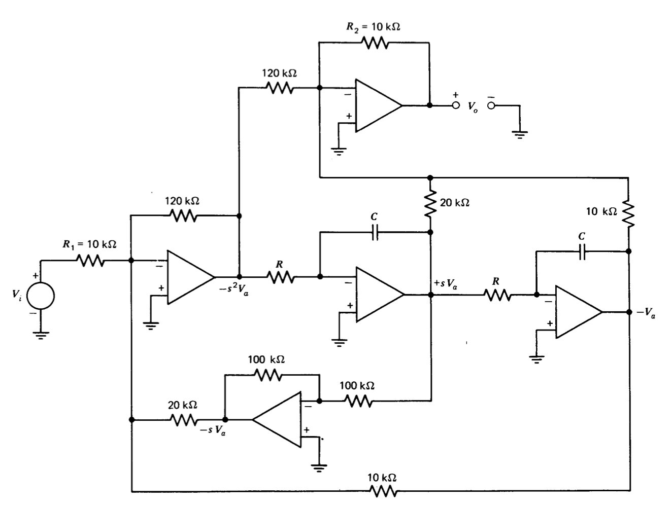
Figure 12.28 Synthesis of second-order Pade approximate to a time delay.

The operational-amplifier synthesis shown in Figure 12.28 provides the required transfer function if \(RC = 1\) second. The reader should convince himself that the liberties taken with inversions and various resistor values do in fact lead to the desired relationship.

Anticipated amplitudes depend on the input-signal level and its spectral content. For example, if a step is applied to the input of the circuit, the magnitude of the signal out of the first amplifier must initially be 12 times as large as the step amplitude, since the outputs of the integrators cannot change instantaneously to subtract from the input-signal level. Note, how­ever, that the input-to-output transfer function of the circuit remains the same for any values of \(R_1 = R_2\). If, for example, 10-V step changes are expected at the input, selection of \(R_1 = R_2 = 120\ k\Omega\) will limit the signal level at the output of the first amplifier to 10 volts while maintaining the correct input-to-output gain.

Figure 12.29 Input and output signals for second-order Pade approximate to a 1-ms time delay. (\(a\)) Sine-wave excitation. (\(b\)) Triangular-wave excitation. (\(c\)) Square-wave excitation.

The circuit shown in Figure 12.28 was constructed using \(R = 100\ k\Omega\) and \(C = 0.01\ \mu F\), values resulting in an approximation to a 1-ms time delay. This choice of time scale is convenient for oscilloscope presentation. The input and output signals for 100-Hz sine-wave excitation are shown in Figure 12.29\(a\). The time delay between these two signals is 1 ms to within instru­mentation tolerances. This performance reflects the prediction of Figure 12.27, since good agreement to 2000 rad/sec or 300 Hz is anticipated for the ap­proximation to a 1-ms delay.

Input and output signals for 100-Hz triangular-wave excitation are com­ pared in Figure 12.29\(b\). The triangular wave contains only odd harmonics, and these harmonics fall off as the square of their frequency. Thus the amplitude of the third harmonic of the triangular wave is approximately 11 % of the amplitude of the fundamental, the amplitude of the fifth harmonic is 4% of the fundamental, while higher harmonics are further attentuated. We notice that the circuit does very well in approximating a 1-ms time delay most of the time. The aberration that results immediately following a change in slope reflects the inability of the circuit to provide proper phase shift to the higher-frequency components.

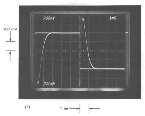
The performance of the circuit when excited with an 100-Hz square wave is shown in Figure 12.29\(c\). The relatively poorer behavior in the vicinity of a transition in this case results from the higher harmonic content of the square wave. (Recall that the square wave contains odd harmonics that fall off only as the first power of the frequency.)