
6.3: Programmable Op Amps
- Page ID
- 3581

As noted in Chapter Five, there is always a trade-off between the speed of an op amp and its power consumption. In order to make an op amp fast (i.e., high slew rate and \(f_{unity}\)), the charging current for the compensation capacitor needs to be fairly high. Other requirements may also increase the current draw of the device. This situation is not unlike that of an automobile where high fuel mileage and fast acceleration tend to be mutually exclusive. Op amps are available that can be set for predetermined performance levels. If the device needs to be very fast, the designer can adjust an external voltage or resistance and optimize the device for speed. At the other end of the spectrum, the device can be optimized for low power draw. Because of their ability to change operational parameters, these devices are commonly called programmable op amps.
Generally, programmable op amps are just like general-purpose op amps, except that they also include a programming input. The current into this pin is called \(I_{set}\). \((I_{set}\) controls a host of parameters including slew rate, \(f_{unity}\), input bias current, standby supply current, and others. A higher value of \(I_{set}\) increases \(f_{unity}\), slew rate, standby current, and input bias current. The value of \(I_{set}\) can be controlled by a simple transistor current source, or even a single resistor in most cases.
One example of a programmable op amp is the Texas Instruments LM4250. The outline of the LM4250 is shown in Figure \(\PageIndex{1}\). Two possible ways of adjusting \(I_{set}\) are shown in Figures \(\PageIndex{2}\) and \(\PageIndex{3}\). A variety of graphs showing the variation of device parameters with respect to \(I_{set}\) are shown in Figure \(\PageIndex{4}\). As an example, assume that \(I_{set}\) = 10 \(\mu\)A and that we're using standard \(\pm\)15 V supplies. At this current, we find that \(f_{unity}\) is 230 kHz, slew rate is 0.21 V/\(\mu\)s, and the standby current draw is 50 \(\mu\)A. The current draw is decidedly lower than that of a 741. This makes the device very attractive for applications where power draw must be kept to a minimum. Battery operated systems generally fall into the low power consumption category. By keeping current drain down, battery life is extended.
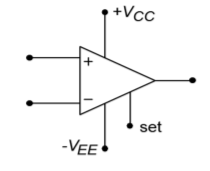
Figure \(\PageIndex{1}\): Basic connections of the LM4250.
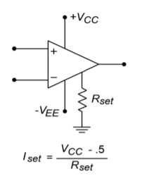
Figure \(\PageIndex{2}\): Programming via resistor.
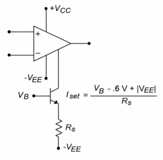
Figure \(\PageIndex{3}\): Programming via voltage.
Perhaps the strongest feature of this class of device is its ability to go into a power down mode. When the device is sitting at idle and not being used, \(I_{set}\) can be lowered, and thus the standby current drops considerably. For example, if \(I_{set}\) for the LM4250 is lowered to 100 nA, standby current drops to under 1 \(\mu\)A. By doing this, the device may only dissipate a few microwatts of power during idle periods. When the op amp again needs to be used for amplification, \(I_{set}\) can be brought back up to a normal level. This form of real time adjustable performance can be instituted with a simple controlling voltage and a transistor current source arrangement as in Figure \(\PageIndex{3}\).
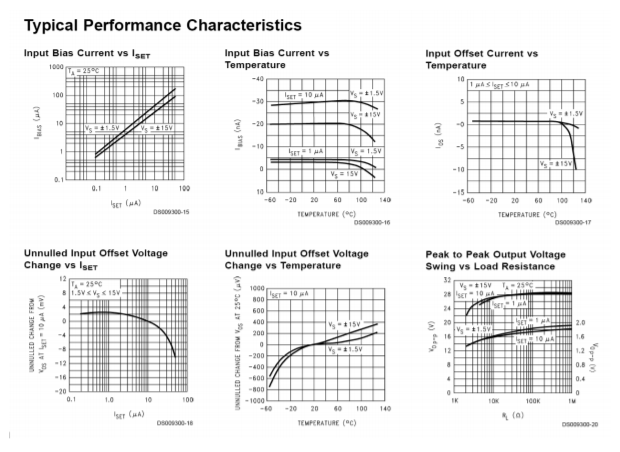
Figure \(\PageIndex{4}\): LM4250 device curves. Reprinted courtesy of Texas Instrutments
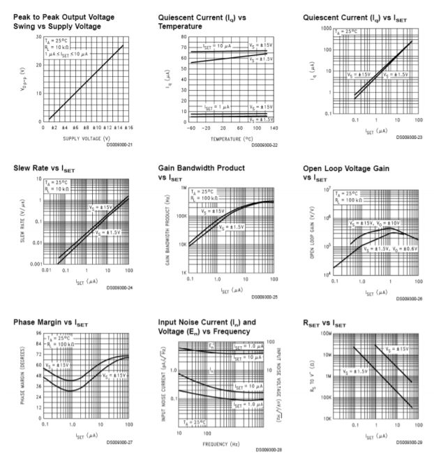
Figure \(\PageIndex{4}\) (continued): LM4250 device curves. Reprinted courtesy of Texas Instrutments
Example \(\PageIndex{1}\)
Determine the power bandwidth for \(V_p = 10 V\) For the circuit of Figure \(\PageIndex{5}\). Also find \(f_2\). \(\pm\)15 V power supplies are used.
In order to find these quantities, we need the slew rate and \(f_{unity}\). These are controlled by \(I_{set}\), so finding \(I_{set}\) is the first order of business.
\[ I_{set} = \frac{V_{CC} − 0.5}{R_{set}} \nonumber \]
\[ I_{set} = \frac{15−0.5}{3MΩ} \nonumber \]
\[ I_{set} = 4.83\mu A \nonumber \]
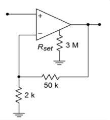
Figure \(\PageIndex{5}\): Circuit for Example \(\PageIndex{1}\).
From the graph “Gain-Bandwidth Product versus \(I_{set}\)” we find that 4.83 \(\mu\)A yields an \(f_{unity}\) of approximately 200 kHz. The graph “Slew Rate versus Iset” yields approximately 0.11 V/\(\mu\)s for the slew rate.
\[ A_{noise} = 1+ \frac{R_f}{R_i} \nonumber \]
\[ A_{noise} = 1+ \frac{50 k}{2 k} \nonumber \]
\[ A_{noise} = 26 \nonumber \]
\[ f_2 = \frac{f_{unity}}{A_{noise}} \nonumber \]
\[ f_2 = \frac{200 kHz}{26} \nonumber \]
\[ f_2 = 7.69kHz \nonumber \]
\[ f_{max} = \frac{SR}{2\pi V_p} \nonumber \]
\[ f_{max} = \frac{0.11V /\mu S}{2 \pi \times 10 V} \nonumber \]
\[ f_{max} = 1.75 kHz \nonumber \]
As you can see, once the set current and associated parameters are found, analysis proceeds as in any general-purpose op amp.