16.6: Open-Loop Transfer Functions and Loci of Roots

Last updated
Save as PDF

Page ID: 7731

\( \newcommand{\vecs}[1]{\overset { \scriptstyle \rightharpoonup} {\mathbf{#1}} } \) \( \newcommand{\vecd}[1]{\overset{-\!-\!\rightharpoonup}{\vphantom{a}\smash {#1}}} \)\(\newcommand{\id}{\mathrm{id}}\) \( \newcommand{\Span}{\mathrm{span}}\) \( \newcommand{\kernel}{\mathrm{null}\,}\) \( \newcommand{\range}{\mathrm{range}\,}\) \( \newcommand{\RealPart}{\mathrm{Re}}\) \( \newcommand{\ImaginaryPart}{\mathrm{Im}}\) \( \newcommand{\Argument}{\mathrm{Arg}}\) \( \newcommand{\norm}[1]{\| #1 \|}\) \( \newcommand{\inner}[2]{\langle #1, #2 \rangle}\) \( \newcommand{\Span}{\mathrm{span}}\) \(\newcommand{\id}{\mathrm{id}}\) \( \newcommand{\Span}{\mathrm{span}}\) \( \newcommand{\kernel}{\mathrm{null}\,}\) \( \newcommand{\range}{\mathrm{range}\,}\) \( \newcommand{\RealPart}{\mathrm{Re}}\) \( \newcommand{\ImaginaryPart}{\mathrm{Im}}\) \( \newcommand{\Argument}{\mathrm{Arg}}\) \( \newcommand{\norm}[1]{\| #1 \|}\) \( \newcommand{\inner}[2]{\langle #1, #2 \rangle}\) \( \newcommand{\Span}{\mathrm{span}}\)\(\newcommand{\AA}{\unicode[.8,0]{x212B}}\)

Let us review and consider again Figure 14.4.1, the general Laplace block diagram for an SISO closed-loop system with feedback. In Section 14.4, we used Figure 14.4.1 to derive the closed-loop transfer function, \(\operatorname{Out}(s) / \operatorname{In}(s)\):

\[C L T F(s)=\frac{G}{1+G H}=\frac{N_{G} D_{H}}{D_{G} D_{H}+N_{G} N_{H}}\label{eqn:16.60} \]

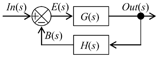
Figure \(\PageIndex{1}\): Laplace block diagram of general closed loop. (Copyright; author via source)

It is common practice also to refer to the ratio \(B(s) / E(s)\) as the open-loop transfer function, which is expressed more completely as

\[\frac{B(s)}{E(s)} \equiv O L T F(s)=G(s) H(s)=\frac{N_{G}(s) N_{H}(s)}{D_{G}(s) D_{H}(s)} \equiv C \times \frac{\prod_{k=1}^{m}\left(s-Z_{k}\right)}{\prod_{k=1}^{n}\left(s-P_{k}\right)}\label{eqn:16.61} \]

In Equation \(\ref{eqn:16.61}\), \(C\) is some physical constant, the finite zeros \(Z_{k}\) of \(\operatorname{OLTF}(s)\) are the roots of \(N_{G}(s) N_{H}(s)=0\), and the poles \(P_{k}\) of \(\operatorname{OLTF}(s)\) are the roots of \(D_{G}(s) D_{H}(s)=0\). [For \(n>m\), there are also \(n-m\) zeros of \(\operatorname{OLTF}(s)\) as \(s \rightarrow \infty\).]

The \(n\)^th degree characteristic polynomial of the closed-loop system is Equation 16.5.16, \(a_{1} \prod_{k=1}^{n}\left(p-p_{k}\right)=0\). Note that the denominator of \(\operatorname{CLTF}(s)\), Equation \(\ref{eqn:16.60}\), equals the denominator plus the numerator of \(\operatorname{OLTF}(s)\), Equation \(\ref{eqn:16.61}\). Therefore, after we divide out coefficient \(a_{1}\), the characteristic equation for closed-loop system poles \(p\) can generally be put into one of the following forms:

\[D_{G}(p) D_{H}(p)+N_{G}(p) N_{H}(p)=0 \Rightarrow\left\{\begin{array}{l}
\text{(a) }\prod_{k=1}^{n}\left(p-P_{k}\right)+c \Lambda=0 \\
\text{(b) }\prod_{k=1}^{n}\left(p-P_{k}\right)+c \Lambda \prod_{k=1}^{m}\left(p-Z_{k}\right)=0
\end{array}\right.\label{eqn:16.62} \]

In Equations \(\ref{eqn:16.62}\), \(c\) is some known physical constant, and \(\Lambda\) is the varying control parameter. The system evaluated by root-locus methods in Section 16.5 includes open-loop poles \(P_k\) (called there the “sub-system poles”), but not any finite open-loop zeros \(Z_k\), so that system’s characteristic equation, Equation 16.5.2, is of form Equation \(\ref{eqn:16.62}\).a. On the other hand, the systems of homework Problems 16.8, 16.9, and 16.10 have both open-loop poles and open-loop zeros, so their characteristic equations have form Equation \(\ref{eqn:16.62}\).b.

Some simple but general features of loci of closed-loop roots can be inferred from Equations \(\ref{eqn:16.62}\). Both equations show clearly that when \(\Lambda=0\), the closed-loop poles are exactly the same as the open-loop poles. At the other extreme, as \(\Lambda\) becomes very large, \(\Lambda \rightarrow \infty\), \(m\) of the loci \(\rightarrow\) the finite open-loop zeros \(Z_{k}\). This is obvious from Equation \(\ref{eqn:16.62}\).b, because the term including the open-loop poles becomes progressively less significant in relative size as the magnitude of \(\Lambda\) increases.

As \(\Lambda \rightarrow \infty\) in Equation \(\ref{eqn:16.62}\).a, in order for an equation of magnitude equality such as Equation 16.5.7, \(r_{1} r_{2} r_{3}=\omega_{b} \Lambda\), to remain satisfied, all \(n\) of the loci of that equation must go to some \(\infty\) locations in the \(p\)-plane. Similarly, as \(\Lambda \rightarrow \infty\) in Equation \(\ref{eqn:16.62}\).b, although \(m\) of the loci terminate at the finite open-loop zeros \(Z_k\), the remaining \(n-m\) loci must go to some \(\infty\) locations in the \(p\)-plane. For both Equations \(\ref{eqn:16.62}\) as \(\Lambda \rightarrow \infty\), the values of the finite open-loop zeros \(Z_k\) and of the open-loop poles \(P_k\) have a secondary influence, so the directions \(\theta_{A}\) in the \(p\)-plane of the \(n - m\) straight-line asymptotes of the \(\Lambda \rightarrow \infty\) loci are the solutions for angles of \(p^{n-m}+c \Lambda=0\), which leads to:

\[\left(r e^{j \theta_{A}}\right)^{n-m}=c \Lambda \exp [j(\pm \pi, \pm 3 \pi, \ldots)] \Rightarrow(n-m) \theta_{A}=\pm \pi, \pm 3 \pi, \ldots \nonumber \]

\[\theta_{A}=\frac{1}{n-m}(\pm \pi, \pm 3 \pi, \ldots)\label{eqn:16.63} \]

However, Equation \(\ref{eqn:16.63}\) neglects the values of \(Z_k\) and \(P_k\), so it implies incorrectly that the asymptotes “radiate” (or “emanate”) from the origin of the \(p\)-plane; in fact, it can be proved (Cannon, 1967, pages 658-659) that all \(n - m\) asymptotes emanate from a point on the real axis defined by the equation:

\[p_{A}=\frac{1}{n-m}\left(\sum_{k=1}^{n} \operatorname{Re}\left[P_{k}\right]-\sum_{k=1}^{m} \operatorname{Re}\left[Z_{k}\right]\right)\label{eqn:16.64} \]

It is useful also to know the directions in which loci “depart” from the open-loop poles as \(\Lambda\) increases from zero. Suppose that we seek the direction (angle) of departure \(\left(\theta_{j}\right)_{d e p}\) of the locus of closed-loop roots from open-loop pole \(P_{j}\). Let us use the following notation: \((\theta P)_{k j}\) is the angle from open-loop pole \(P_{k}\) to open-loop pole \(P_{j}\); and \((\theta Z)_{k j}\) is the angle from open-loop zero \(Z_k\) to open-loop pole \(P_{j}\). Provided that all of the open-loop poles and zeros are single (not repeated or multiple) roots, then the required angle is calculated from the equation (Cannon, 1967, pages 660-661):

\[\left(\theta_{j}\right)_{d e p}=\pi-\sum_{k=1 \atop k \neq j}^{n}(\theta P)_{k j}+\sum_{k=1}^{m}(\theta Z)_{k j}\label{eqn:16.65} \]

We use Section 16.5’s numerical example to illustrate the information about loci of roots that is provided by open-loop poles; that example is a 3^rd order system for which \(n=3\) and \(m=0\). From Equation 16.5.2 with \(\Lambda=0\), the open-loop poles are \(p_{1}=0\) s^-1, \(p_{2}=-100\) s^-1, and \(p_{3}=-300\) s^-1. These open-loop poles are marked by \(\times\)’s on Figure \(\PageIndex{2}\). There are no open-loop zeros, so as \(\Lambda \rightarrow \infty\), the three loci must go to some \(\infty\) locations in the \(p\)-plane; the directions of the lines asymptotic to these loci are given by Equation \(\ref{eqn:16.63}\) as \(\theta_{A}=\pm \pi / 3\) and \(\theta=\pi\). The point on the real axis from which all three asymptotes emanate is given by Equation \(\ref{eqn:16.64}\) as \(p_{A}=(0-100-300) / 3=-133\frac{1}{3}\) s^-1. The asymptotes are the straight dashed lines on Figure \(\PageIndex{2}\). Equation \(\ref{eqn:16.65}\) gives the angles of departure from open-loop poles as \(\left(\theta_{1}\right)_{d e p}=\pi-(0+0)=\pi\), \(\left(\theta_{2}\right)_{d e p}=\pi-(\pi+0)=0\), and \(\left(\theta_{3}\right)_{d e p}=\pi-(\pi +\pi)=-\pi\). These angles of departure are represented on Figure \(\PageIndex{2}\) by short, bold arrows. Although the directions of departure for this particular system are either due east or due west, this is not always the case; for systems in general, a direction of departure can be any angle.

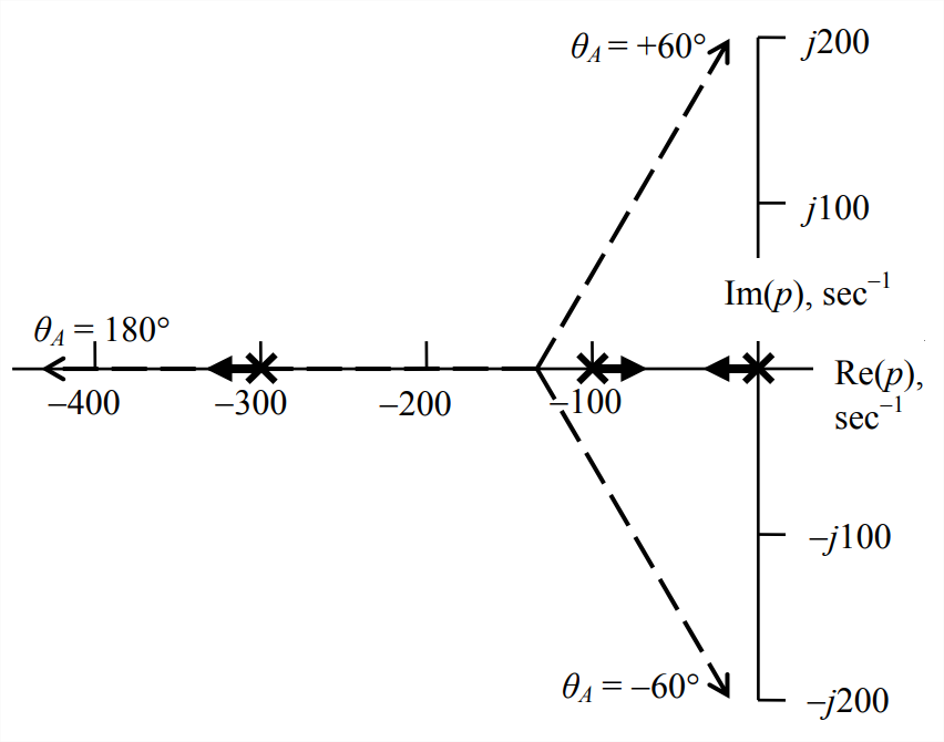
Figure \(\PageIndex{2}\): Example of information about loci of roots that is provided by the open-loop poles. (Copyright; author via source)

We can make educated guesses as to the appearance of the completed diagram of root loci, even from the incomplete diagram Figure \(\PageIndex{2}\). First, it seems likely that the locus originating (i.e., for \(\Lambda=0\)) at open-loop pole \(p_{3}=-300\) s^-1 just proceeds westerly along the asymptote \(\theta_{A}=\pi\), without straying away from the \(\operatorname{Re}(p)\) axis. That being the case, then the loci originating from the open-loop poles \(p_{1}=0\) s^-1 and \(p_{2}=-100\) s^-1 must initially approach each other, then come together somewhere between \(p_{1}\) and \(p_{2}\), and then break away from the \(\operatorname{Re}(p)\) axis and become the complex conjugate pair of curves to which the asymptotes \(\theta_{A}=\pm \pi / 3\) are tangent as \(\Lambda \rightarrow \infty\). Certainly, the incomplete diagram Figure \(\PageIndex{2}\) is qualitatively similar to the exact diagram Figure 16.5.5, and Figure \(\PageIndex{2}\) even includes some of the same significant quantitative information.

When you use software to determine loci of roots, you should also make the easy calculations presented in this section based upon open-loop poles and zeros. If the software calculations match yours, then this check will validate (partially, at least) that the software is correct and that you are using it correctly.