16.5: Loci of Roots for Third Order Systems

In Section 16.4, we used the quadratic formula to evaluate easily the loci of roots for 2^nd order systems. It is more typical in practice, however, that engineering systems have higher orders than 2^nd order, so that determining loci of roots requires repeatedly solving polynomial equations of 3^rd and higher degrees, which can be a challenging task. This section introduces by example the methods of solution for higher-order systems that are commonly used in practice.

For this example, we consider again the system described in Section 16.3 (Figures 16.3.1, 16.3.2, and 16.3.3), a rotor position-feedback control system with a 1^st order low-pass filter in the feedback branch. Closed-loop transfer function Equation 16.3.9 gives the 3^rd degree characteristic equation in two different algebraic forms, one of which is

\[\operatorname{Den}(p)=a_{1} p^{3}+a_{2} p^{2}+a_{3} p+a_{4}=p^{3}+\left(\frac{1}{\tau_{L}}+\frac{c_{\theta}}{J}\right) p^{2}+\frac{c_{\theta}}{J} \frac{1}{\tau_{L}} p+\frac{K_{a} K_{\theta}}{J \tau_{L}}=0\label{eqn:16.51a} \]

In Section 16.3, we held constant rotor inertia \(J\), viscous damping constant \(c_{\theta}\) of the bearings, and time constant \(\tau_{L}\) of the 1^st order low-pass filter, all positive values; in particular, we chose for numerical evaluation the values \(c_{\theta} / J=100\) s^-1, and, for the filter break frequency, \(\omega_{b} \equiv 1 / \tau_{L}=300\) rad/s. We allowed the value of product \(K_{a} K_{\theta}\) of control system sensitivities to vary. Using Routh’s criteria, we determined the lower and upper stability boundaries for the parameter \(K_{a} K_{\theta} / J \equiv \Lambda\): the system is positively stable provided that \(0<\Lambda<40,000\) s^-2.

Now, let us conduct a more detailed evaluation of stability by calculating and plotting the loci of roots as \(\Lambda\) varies, using the same numerical values of the other constants as in Section 16.3. We solve numerically for the roots of polynomial Equation \(\ref{eqn:16.51a}\) using MATLAB’s root operation: for each value of \(\Lambda\), the input is the array of coefficients \(\left[\begin{array}{llll}
a_{1} & a_{2} & a_{3} & a_{4}
\end{array}\right]\), and the output is the \(3 \times 1\) matrix of roots. We will calculate and plot the loci of roots twice: first, for a set of \(\Lambda\) values that we choose (guess) somewhat arbitrarily to encompass the entire possible range of practical interest; second, for another set of \(\Lambda\) values that are refined, based upon the results of the first pass, to focus on the specific roots of greatest practical significance.

For the first pass, we vary \(\Lambda\) from −30,000 s^-2 to +70,000 s^-2 in increments of 10,000 s^-2. The following is a MATLAB script M-file that computes the roots of polynomial Equation \(\ref{eqn:16.51a}\) repeatedly over these values of \(\Lambda\), then prints the input and output values in a table, then plots the loci of roots:

%MATLABdemo163.m

%Stability of a damped rotor with low-pass-filtered position feedback

%Loci of roots

wb=300;covrJ=100;a2=wb+covrJ;a3=wb*covrJ;

Lm=[-3 -2 -1 0 1 2 3 4 5 6 7]*1.0e4;Np=length(Lm);

for i=1:Np;

a4=Lm(i)*wb;

p(i,1:3)=roots([1 a2 a3 a4]).';

end

nc=1:Np;anout=[nc' Lm' p];

disp('Roots #, Lambda, p'),disp(anout)

plot(p,'kx'),grid,xlabel('Real part of pole (sec^-^1)')

ylabel('Imag part of pole (sec^-^1)')

title('Loci of roots of a 3^r^d order system as \Lambda varies')

The command to execute the M-file, and the resulting tabular output follows:

>> MATLABdemo163

Roots #, Lambda, p

1.0e+004 *

0.0001 -3.0000 -0.0253 + 0.0141i -0.0253 - 0.0141i 0.0107

0.0002 -2.0000 -0.0242 + 0.0111i -0.0242 - 0.0111i 0.0085

0.0003 -1.0000 -0.0227 + 0.0056i -0.0227 - 0.0056i 0.0055

0.0004 0 0 -0.0300 -0.0100

0.0005 1.0000 -0.0337 -0.0031 + 0.0089i -0.0031 - 0.0089i

0.0006 2.0000 -0.0363 -0.0019 + 0.0127i -0.0019 - 0.0127i

0.0007 3.0000 -0.0383 -0.0008 + 0.0153i -0.0008 - 0.0153i

0.0008 4.0000 -0.0400 -0.0000 + 0.0173i -0.0000 - 0.0173i

0.0009 5.0000 -0.0415 0.0007 + 0.0190i 0.0007 - 0.0190i

0.0010 6.0000 -0.0428 0.0014 + 0.0205i 0.0014 - 0.0205i

0.0011 7.0000 -0.0440 0.0020 + 0.0217i 0.0020 - 0.0217i

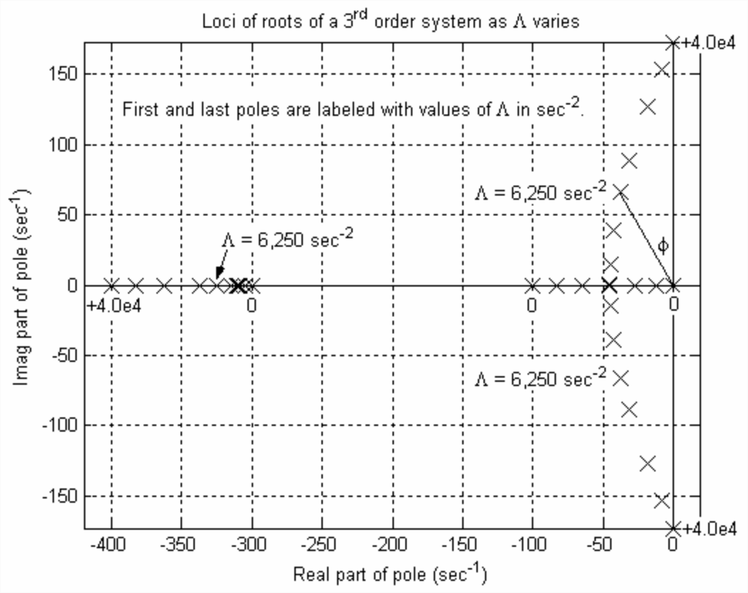
The associated loci-of-roots plot (after use of MATLAB’s editing features for annotation and graphical enhancement) is Figure \(\PageIndex{1}\).

Figure \(\PageIndex{1}\): First-pass loci of roots of Equation \(\ref{eqn:16.51a}\) for varying control parameter \(\Lambda=K_{a} K_{\theta} / J\). (Copyright; author via source)

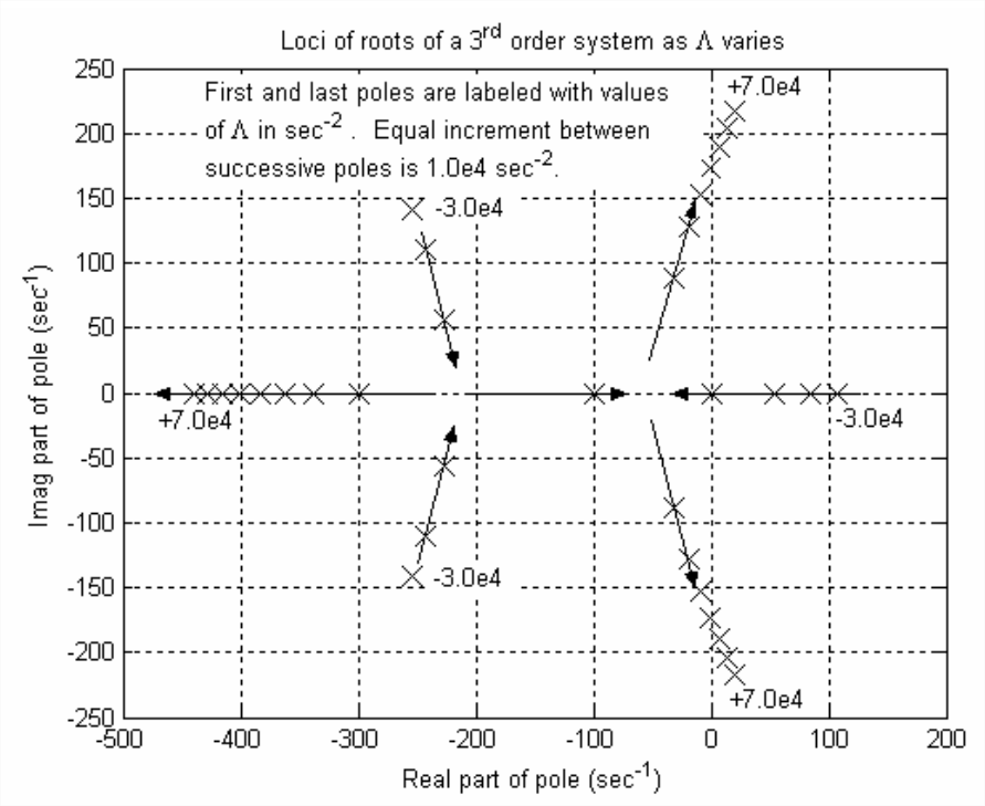
We infer from Figure \(\PageIndex{1}\) the following relevant information. For \(\Lambda<0\), the system has an unstable pole associated with monotonic exponentially growing time response; we already knew from Routh that the system is unstable for \(\Lambda<0\), but Routh did not reveal the type of response. For \(\Lambda=0\), the poles are all real and have the values 0, −100, and −300 s^-1. This is also obvious in the alternate algebraic form of the 3^rd degree characteristic equation that comes from closed-loop transfer function Equation 16.3.9:

\[\operatorname{Den}(p)=p\left(p+c_{\theta} / J\right)\left(p+\omega_{b}\right)+\omega_{b} \Lambda=0\label{eqn:16.51b} \]

From Equation \(\ref{eqn:16.51a}\) with \(\Lambda=0\), the poles are clearly \(p_1 = 0\), \(p_{2}=-c_{\theta} / J=-100\) s^-1, and \(p_3 = -\omega_{b} \equiv-1 / \tau_{L}=-300\) s^-1. The arrows on Figure \(\PageIndex{1}\) indicate the directions of loci as \(\Lambda\) increases. The arrows show that there is a break-in point (as defined on Figure 16.4.1) for \(\Lambda\) somewhere in the range \(-10,000 s ^{-2}<\Lambda<0\), and a break-away point for \(\Lambda\) somewhere in the range \(0<\Lambda<+10,000\) s^-2. For future reference, let us denote the break-away value of \(\Lambda\) as \(\Lambda_{b a}\), which is not yet determined. We also observe from Figure \(\PageIndex{1}\) and the tabulated roots that the upper boundary of stability (with purely complex roots, \(p_{2,3}=\pm j 173\) rad/s) is \(\Lambda=40,000\) s^-2, and that the time response is oscillatory for values of \(\Lambda\) in the vicinity of the upper boundary; we knew from Routh the value of the upper boundary, but not the type of response. Moreover, since the real pole for \(\Lambda>\Lambda_{b a}\) is associated with heavily damped exponential decay, the complex loci for \(\Lambda>\Lambda_{b a}\) of Figure \(\PageIndex{1}\) suggest that the time response is primarily oscillatory for \(\Lambda>\Lambda_{b a}\). See Figure 16.3.3 for examples of this primarily oscillatory response. For \(\Lambda>\Lambda_{b a}\), this system has a heavily damped exponential mode of response and a lightly damped oscillatory mode, and the latter, with poles closest to the imaginary axis, is the dominant mode.

Now let us refine the loci-of-roots calculation, using a new set of \(\Lambda\) values that would be of greatest practical interest. This set probably would consist of values for which the system is stable, namely \(0<\Lambda<40,000\) s^-2. The value \(\Lambda_{b a}\) is significant: it is the boundary between a system (with \(0<\Lambda<\Lambda_{b a}\)) for which all transient response is decaying exponential and a system (with \(\Lambda_{b a}<\Lambda\)) for which the dominant transient response is oscillatory. We certainly could choose the refined set of Λ values by numerical trial and error, letting MATLAB do most of the work. However, this situation provides the opportunity for introduction of a theoretical and more systematic approach, which we shall consider next. This approach is general, but our limited objective in this introduction will be to determine theoretically only the upper boundary of stability, \(\Lambda \equiv \Lambda_{u b}\), and the break-away value \(\Lambda_{b a}\).

This approach is based upon form Equation \(\ref{eqn:16.51b}\) of the characteristic equation, which we re-write as

\[p\left(p+c_{\theta} / J\right)\left(p+\omega_{b}\right)=-\omega_{b} \Lambda\label{eqn:16.52} \]

It is important that the sub-system poles are separated into factors on the left-hand side of Equation \(\ref{eqn:16.52}\). Each factor is a complex number, in general, and it can be expressed in complex polar form, as described in Section 2.1. It is helpful to regard each factor as a two-dimensional complex vector with its tail at the sub-system pole, so that we write

\[p=p-0 \equiv r_{1} e^{j \theta_{1}}, p+c_{\theta} / J=p-\left(-c_{\theta} / J\right) \equiv r_{2} e^{j \theta_{2}}, p+\omega_{b}=p-\left(-\omega_{b}\right) \equiv r_{3} e^{j \theta_{3}}\label{eqn:16.53} \]

The real right-hand side of Equation \(\ref{eqn:16.52}\) also is written in polar form: \(-\omega_{b} \Lambda= \omega_{b} \Lambda \exp [j(\pm \pi, \pm 3 \pi, \ldots)]\). Therefore, the entire characteristic equation is expressed in the following polar form, which any root must satisfy:

\[r_{1} e^{j \theta_{1}} \times r_{2} e^{j \theta_{2}} \times r_{3} e^{j \theta_{3}}=r_{1} r_{2} r_{3} e^{j\left(\theta_{1}+\theta_{2}+\theta_{3}\right)}=\omega_{b} \Lambda \exp [j(\pm \pi, \pm 3 \pi, \ldots)]\label{eqn:16.54} \]

Figure \(\PageIndex{2}\) (Copyright; author via source)

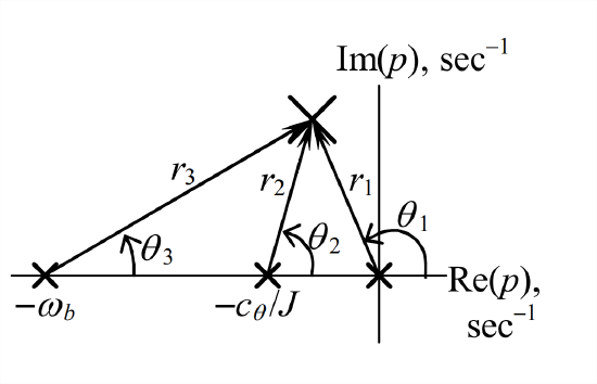
The drawing above is a graphical representation of both the polar vectors of Equation \(\ref{eqn:16.53}\) and characteristic equation Equation \(\ref{eqn:16.54}\). The small \(\times\)’s are the sub-system poles, at which the tails of the complex vectors are located. The large \(\mathbf{X}\) is a pole of the complete system, i.e., a root of Equation \(\ref{eqn:16.51b}\), and a value that satisfies Equation \(\ref{eqn:16.54}\). Complex equation Equation \(\ref{eqn:16.54}\) includes two real equations, both of which must be satisfied by any system pole. The first equation is the equality of angles on the two sides of Equation \(\ref{eqn:16.54}\):

\[\theta_{1}+\theta_{2}+\theta_{3}=\pm \pi, \pm 3 \pi, \ldots\label{eqn:16.55} \]

The second equation is the equality of magnitudes:

\[r_{1} r_{2} r_{3}=\omega_{b} \Lambda \Rightarrow \Lambda=\frac{r_{1} r_{2} r_{3}}{\omega_{b}}\label{eqn:16.56} \]

For our first application of this approach, let us use Equation \(\ref{eqn:16.55}\) to find the pole \(j \omega_{d}\) at the upper stability boundary \(\Lambda_{u b}\), and then Equation \(\ref{eqn:16.56}\) to find the value of \(\Lambda_{u b}\) itself. The pole is shown on the drawing at right. We have by definition for this stability boundary: \(r_{1}=\omega_{d}\) and \(\theta_{1}=\pi / 2\). Therefore, Equation \(\ref{eqn:16.55}\) gives \(\theta_{2}+\theta_{3}=\pi / 2\). [We rule out the other possibilities \(-\pi, \pm 3 \pi, \ldots\) in Equation \(\ref{eqn:16.55}\) just by inspecting the figure.] Some trigonometry is required now. Angle \(\alpha\) between the arrowheads of \(r_1\) and \(r_2\) is labeled on the drawing. Angles \(\alpha\) and \(\theta_{3}\) are the complementary acute angles of a right triangle, so we have also \(\alpha+\theta_{3}=\pi / 2\). Therefore, \(\alpha=\theta_{2}\). Hence, we find \(\omega_{d}\) by equating the tangents of the two similar right triangles:

Figure \(\PageIndex{3}\) (Copyright; author via source)

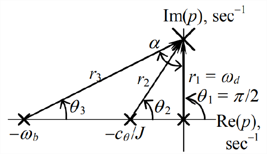
\[\tan \theta_{2}=\frac{\omega_{d}}{c_{\theta} / J}=\tan \alpha=\frac{\omega_{b}}{\omega_{d}} \Rightarrow \omega_{d}=\sqrt{\omega_{b} \frac{c_{\theta}}{J}}=\sqrt{300 \mathrm{s}^{-1} \times 100 \mathrm{s}^{-1}}=173.2 \frac{\mathrm{rad}}{\mathrm{s}} \nonumber \]

Having \(\omega_{d}=r_{1}\), we can use the theorem of Pythagoras to find \(r_{2}=\sqrt{\omega_{d}^{2}+\left(c_{\theta} / J\right)^{2}}=\sqrt{\omega_{b}\left(c_{\theta} / J\right)+\left(c_{\theta} / J\right)^{2}}\) and \(r_{3}=\sqrt{\omega_{d}^{2}+\omega_{b}^{2}}=\sqrt{\omega_{b}\left(c_{\theta} / J\right)+\omega_{b}^{2}}\). Finally, we find \(\Lambda_{u b}\) by applying Equation \(\ref{eqn:16.56}\), which, after a little algebra, gives

\[\Lambda_{u b}=\frac{r_{1} r_{2} r_{3}}{\omega_{b}}=\omega_{b} \frac{c_{\theta}}{J}+\left(\frac{c_{\theta}}{J}\right)^{2}=300 \mathrm{s}}^{-1} \times 100 \mathrm{s}}^{-1}+\left(100 \mathrm{s}}^{-1}\right)^{2}=40,000 \mathrm{s}}^{-2} \nonumber \]

This result for \(\Lambda_{u b}\) is, of course, identical to the upper boundary found by Routh’s criteria in Equation 16.3.13.

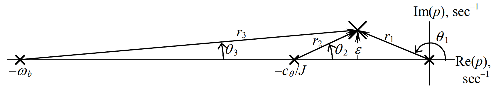
For a more subtle application of this theoretical approach, let us: first, use Equation \(\ref{eqn:16.55}\) to find the value of the two identical poles at the break-away point, which is evident on Figure \(\PageIndex{1}\) (on the real axis, somewhere between the origin and \(-c_{\theta} / J=-100\) s^-1); and then, use Equation \(\ref{eqn:16.55}\) to find the associated value of \(\Lambda_{b a}\). It is obvious that Equation \(\ref{eqn:16.55}\) is satisfied identically right at the break-away point, where \(\theta_{1}=\pi\) and \(\theta_{2}=\theta_{3}=0\), so this does not provide any useful information. But Equation \(\ref{eqn:16.55}\) must apply also for all other points on the loci of roots, in particular now, for points that are close to the break-away point; this fact will lead to a useful result. Suppose that \(\Lambda\) is just slightly greater than \(\Lambda_{b a}\) so that one of the complex poles is a small distance \(\mathcal{E}\) above the break-away point on the real axis, as shown on the drawing below. As \(\mathcal{E}\) shrinks but remains \(> 0\), the acute angles between the sub-system radii and the real axis become very small, so we can use in Equation \(\ref{eqn:16.55}\) the approximation \(\theta \approx \sin \theta\). Hence, Equation \(\ref{eqn:16.55}\) gives

\[\theta_{1}+\theta_{2}+\theta_{3}=\left(\pi-\frac{\varepsilon}{r_{1}}\right)+\frac{\varepsilon}{r_{2}}+\frac{\varepsilon}{r_{3}}=\pi \Rightarrow \varepsilon\left(-\frac{1}{r_{1}}+\frac{1}{r_{2}}+\frac{1}{r_{3}}\right)=0 \nonumber \]

This equation must be valid even if \(\mathcal{E}\) is very small but non-zero, so we conclude that

\[-\frac{1}{r_{1}}+\frac{1}{r_{2}}+\frac{1}{r_{3}}=0=\frac{-r_{2} r_{3}+r_{1} r_{3}+r_{1} r_{2}}{r_{1} r_{2} r_{3}} \Rightarrow-r_{2} r_{3}+r_{1} r_{3}+r_{1} r_{2}=0 \nonumber \]

Figure \(\PageIndex{4}\) (Copyright; author via source)

In the limit as the pole goes to the break-away point on the real axis, \(\varepsilon=0\), the radii are related as \(r_{1}+r_{2}=c_{\theta} / J\) and \(r_{1}+r_{3}=\omega_{b}\). Substituting into the equation above to eliminate \(r_2\) and \(r_3\) gives \(-r_{2} r_{3}+r_{1}\left(r_{3}+r_{2}\right)=-\left(c_{\theta} / J-r_{1}\right)\left(\omega_{b}-r_{1}\right)+r_{1}\left(\omega_{b}-r_{1}+c_{\theta} / J-r_{1}\right)= 0\), and this leads, after some algebra, to a quadratic equation in unknown \(r_1\):

\[3 r_{1}^{2}-2\left(\omega_{b}+\frac{c_{\theta}}{J}\right) r_{1}+\omega_{b} \frac{c_{\theta}}{J}=0 \nonumber \]

Solving for \(\r_1\) with the quadratic formula gives

\[r_{1}=\frac{1}{3}\left[\left(\omega_{b}+\frac{c_{\theta}}{J}\right) \pm \sqrt{\left(\omega_{b}+\frac{c_{\theta}}{J}\right)^{2}-3 \omega_{b} \frac{c_{\theta}}{J}}\right] \nonumber \]

Substituting into this equation \(\omega_{b}=300\) s^-1 and \(c_{\theta} / J=100\) s-1 gives the roots 221.53 and 45.14 s^-1, with the latter root corresponding to the break-away pole that we seek between the origin and −100 s^-1 on the real axis, i.e., \(r_{1}=45.14\) s^-1. Then Equation \(\ref{eqn:16.56}\) gives the associated value of the varying control parameter:

\[\Lambda_{b a}=\frac{r_{1} r_{2} r_{3}}{\omega_{b}}=\frac{r_{1}\left(c_{\theta} / J-r_{1}\right)\left(\omega_{b}-r_{1}\right)}{\omega_{b}}=2,103.77 \mathrm{s} ^{-2} \nonumber \]

The approach used above to determine theoretically the stability-upper-bound and break-away values of the varying control parameter \(\Lambda\), based upon Equations \(\ref{eqn:16.52}\)-\(\ref{eqn:16.56}\), is a small portion of an extensive set of procedures for completely determining loci of roots, which is known as the root-locus method. Walter R. Evans (1920-1999, American electrical engineer) developed and published this elegant method around 1950. Using the root-locus method, an experienced engineer can develop quickly, without the need for a digital computer, complete loci of roots, even for systems of somewhat higher order. For about a quarter-century after this method became widely known, the slide rule was still an engineer’s primary computational tool, and the root-locus method profoundly influenced the design and analysis of control systems during that era. Now that digital computers and highly specialized software are readily available, Evans’ root-locus method is no longer so essential if you need only to analyze a given system. However, if you want to design control systems logically and efficiently, then the concepts underlying Evans’ method, represented in this example by Equations \(\ref{eqn:16.52}\)-\(\ref{eqn:16.56}\), will be extremely valuable. Details of Evans’ method are available in many references, one of the clearest and most complete being Cannon, 1967, Sections 11.8 and 11.9 and Chapter 21.

Let us return now to the task of choosing a refined set of \(\Lambda\) values and using MATLAB to calculate and graph loci of roots for this refined set. We specify that this set consists of values for which the system is stable, \(0<\Lambda<40,000\) s^-2, with particular emphasis on the range of values associated with the dominant oscillatory mode of response, \(\Lambda_{b a}<\Lambda<40,000\) s^-2. Therefore, the value \(\Lambda_{b a}=2,103.77\) s^-2 calculated above is useful, and is included in the refined set of \(\Lambda\) values. The other values are chosen by trial and error to produce moderately uniform spacing between the complex poles in the \(p\)-plane; the complete set, in ascending order is \(\Lambda =\) 0, 1,000, 1,800, \(\Lambda_{b a}\), 2,300, 3,500, 6,250, 10,000, 20,000, and 40,000 s^-2. Except for this different set of \(\Lambda\) values, the MATLAB script M-file is the same as that which produced Figure \(\PageIndex{1}\). The command to execute the M-file, and the resulting tabular output follows:

>> MATLABdemo164

Roots #, Lambda, p

1.0e+004 *

0.0001 0 0 -0.0300 -0.0100

0.0002 0.1000 -0.0305 -0.0083 -0.0012

0.0003 0.1800 -0.0308 -0.0064 -0.0027

0.0004 0.2104 -0.0310 -0.0045 + 0.0000i -0.0045 - 0.0000i

0.0005 0.2300 -0.0311 -0.0045 + 0.0015i -0.0045 - 0.0015i

0.0006 0.3500 -0.0315 -0.0042 + 0.0039i -0.0042 - 0.0039i

0.0007 0.6250 -0.0326 -0.0037 + 0.0066i -0.0037 - 0.0066i

0.0008 1.0000 -0.0337 -0.0031 + 0.0089i -0.0031 - 0.0089i

0.0009 2.0000 -0.0363 -0.0019 + 0.0127i -0.0019 - 0.0127i

0.0010 3.0000 -0.0383 -0.0008 + 0.0153i -0.0008 - 0.0153i

0.0011 4.0000 -0.0400 -0.0000 + 0.0173i -0.0000 - 0.0173i

The associated loci-of-roots plot, Figure \(\PageIndex{5}\), is on the next page. MATLAB’s editing features for annotation and graphical enhancement were used on Figure \(\PageIndex{5}\). In particular, the axes were set to be “equal,” which means in this case that the \(x\) axis [i.e., \(\operatorname{Re}(p)\)] and the \(y\) axis [i.e., \(\operatorname{Im}(p)\)] have exactly the same linear scale.

Figure \(\PageIndex{5}\): Refined loci of roots of Equation \(\ref{eqn:16.51a}\) for varying control parameter Λ = KaKθ ⁄ J. (Copyright; author via source)

The roots on Figure \(\PageIndex{5}\) for one example value, \(\Lambda=6,250\) s^-2, are labeled in order to illustrate calculation of basic 1^st order and 2^nd order parameters for a higher-order system. The real root is \(p_{1}=-326\) s^-1 (taken approximately from Figure \(\PageIndex{5}\), but more precisely from the table of roots on the previous page). The associated 1^st order time constant is \(\tau_{1}=-1 / p_{1}=3.07 \mathrm{e}-3\) s = 3.07 ms. The imaginary roots for \(\Lambda=6,250\) s−2 are \(p_{2,3}=-37 \pm j 66\) s^-1, and the angle labeled on Figure \(\PageIndex{5}\) is \(\phi \approx 30^{\circ}\) (for its relevance, see Figure \(\PageIndex{5}\)). The associated 2^nd order response parameters are: time constant \(\tau_{2}= -1 / \operatorname{Re}\left(p_{2,3}\right)=27\) ms (much longer than \(\tau_1\)); frequency \(\omega_{d}=\operatorname{Im}\left(p_{2}\right)=66\) rad/s; and damping ratio \(\zeta=\sin \phi \approx 0.5\) We can use MATLAB’s poles to calculate more precisely the damping ratio associated with a stable complex pole, \(p_{k}=\sigma_{k}+j \omega_{k}\) (the notation of Section 16.1), by recognizing that \(\sigma_{k}=\operatorname{Re}\left(p_{k}\right) \equiv-\left(\zeta \omega_{n}\right)_{k}\) and \(\omega_{k}= \operatorname{Im}\left(p_{k}\right) \equiv\left(\omega_{d}\right)_{k}\), and that (dropping the \(k\) subscripts temporarily) \(\omega_{d}^{2}=\omega_{n}^{2}-\left(\zeta \omega_{n}\right)^{2}\):

\[\zeta^{2}=\frac{\left(\zeta \omega_{n}\right)^{2}}{\omega_{n}^{2}}=\frac{\left(\zeta \omega_{n}\right)^{2}}{\left(\zeta \omega_{n}\right)^{2}+\omega_{d}^{2}} \equiv \frac{\sigma^{2}}{\sigma^{2}+\omega^{2}}=\frac{1}{1+(\omega / \sigma)^{2}} \nonumber \]

Therefore (restoring the \(k\) subscripts), the damping ratio is

\[\zeta_{k}=\frac{1}{\sqrt{1+\left(\omega_{k} / \sigma_{k}\right)^{2}}}\label{eqn:16.57} \]

Applying Equation \(\ref{eqn:16.57}\) for \(\Lambda=6,250\) s^-2 gives \(\zeta_{2}=1 / \sqrt{1+(66 / 37)^{2}}=0.49\).

The calculations in the previous paragraph suggest the following question: why does this 3^rd order system have one real pole that corresponds to monotonic exponential 1^st order response, and a pair of complex conjugate poles that correspond to damped oscillatory 2^nd order response? In fact, this is a simple example of an important general property of linear time-invariant systems. Every LTI system has modes of response that are associated with its poles, the roots of the system’s characteristic equation. We show this by re-writing characteristic equation Equation 16.3.1 in the general factored form:

\[\operatorname{Den}(p)=a_{1} p^{n}+a_{2} p^{n-1}+\cdots+a_{n} p+a_{n+1}=a_{1} \prod_{k=1}^{n}\left(p-p_{k}\right)=0\label{eqn:16.58} \]

where the \(\prod_{k=1}^{n}\) symbol denotes multiplication of \(n\) terms. Since all coefficients \(a_{k}\) are real, this equation can always be factored into 1^st order terms with real poles and 2^nd order terms with complex conjugate poles for which \(\left|\zeta_{j}\right|<1\):

\[\frac{1}{a_{1}} \operatorname{Den}(p)=\prod_{k=1}^{n}\left(p-p_{k}\right)=\ldots\left(p-p_{i}\right) \ldots\left(p^{2}+2 \zeta_{j} \omega_{j} p+\omega_{j}^{2}\right) \ldots\label{eqn:16.59} \]

It might be conceptually clearest to think of the modes in terms of response to initial conditions, without the complication of forcing inputs. The mode of IC response associated with any real pole [\(p_{i}\) in Equation \(\ref{eqn:16.59}\)] is monotonic exponential, exactly that of a basic 1^st order system. The mode of IC response associated with any pair of complex conjugate poles [\(-\zeta_{j} \omega_{j} \pm j \omega_{j} \sqrt{1-\zeta_{j}^{2}}\) in Equation \(\ref{eqn:16.59}\)] is oscillation modulated by an exponential envelope, exactly that of a basic 2^nd order system for which \(|\zeta|<1\). The total time response of an LTI system to initial conditions and forcing inputs is the superposition of the responses of all of its individual 1^st order and 2^nd order modes. If the response is stable, then the greatest contributors to this total response typically are a few, at most, dominant modes, those whose poles are closest to the imaginary axis.

The modes of vibration introduced in Section 7.6 and Chapter 12 represent a special case of the more general modes of response discussed in the previous paragraph. An undamped structural system of the type considered in Chapter 12 always has even order (i.e., \(n=2,4,6, \ldots\)), so that its characteristic equation has an even number of roots. These roots appear in purely imaginary conjugate pairs, each pair for a particular mode of vibration; the absolute value of any root is the natural frequency of that particular mode.

Before proceeding, we should observe a general feature of loci-of-roots diagrams. The poles are either real or, if complex, appear in conjugate pairs, as is expressed by Equation \(\ref{eqn:16.59}\). Therefore, loci-of-roots diagrams are always symmetric about the \(\operatorname{Re}(p)\) axis. This symmetry is evident in Figures 16.4.1, \(\PageIndex{1}\), and \(\PageIndex{5}\).