16.4: Loci of Roots for Second Order Systems

Let us seek both the type of response and the degree of stability, by directly solving for the roots of the characteristic equation \(\operatorname{Den}(p)=0\) [i.e., the poles of \(TF(s)\) or \(CLTF(s)\), whichever is appropriate]. Further, we will observe how these roots vary as some particular system parameter is changed. The graphical representation of this variation in the complex \(p\)-plane is known commonly as \(locus of roots\); however, systems of 2^nd and higher orders always have multiple roots, so it is more correct to use the Latin plural: loci of roots. Stability analysis using loci of roots is more general than the basic Routh’s criteria, and more informative about the character of a system and the nature of its stability.

We begin by studying the roots of any 2^nd order system. This will be instructive and will also establish the basis for interpretation of loci-of-roots graphs for LTI systems of higher order. The characteristic equation of any 2^nd order system can be expressed as:

\[\operatorname{Den}(p)=p^{2}+2 \zeta \omega_{n} p+\omega_{n}^{2}=0\label{eqn:16.47} \]

Some examples of 2^nd order system transfer functions that lead to Equation \(\ref{eqn:16.47}\) are Equations 10.2.3, 10.4.4, 13.2.3, 14.5.4, 15.2.19, and 15.4.3. We are accustomed to studying stable systems for which \(\zeta\) and \(\omega_{n}^{2}\) are positive values. However, these parameters are not necessarily always positive in systems; they can be negative, especially for feedback control systems and for self-excited systems. An example of a self-excited system is a flexible wing in an airstream, as discussed in Examples 11.3.2 and 11.3.3 of Section 11.3.

First, let us study the roots of Equation \(\ref{eqn:16.47}\) when \(\zeta\) varies, in both magnitude and sign, while \(\omega_{n}\) is fixed and positive, \(\omega_{n}>0\). Solving first for \(|\zeta| \geq 1\), using the quadratic formula, gives the two real-valued poles:

\[p_{1,2}=-\zeta \omega_{n} \pm \omega_{n} \sqrt{\zeta^{2}-1}\label{eqn:16.48a} \]

For \(|\zeta| \leq 1\), the poles are the complex conjugate pair:

\[p_{1,2}=-\zeta \omega_{n} \pm j \omega_{n} \sqrt{1-\zeta^{2}} \equiv-\zeta \omega_{n} \pm j \omega_{d}\label{eqn:16.48b} \]

Figure \(\PageIndex{1}\) shows the loci of roots Equations \(\ref{eqn:16.48a}\) and \(\ref{eqn:16.48b}\) as \(\zeta\) varies from more negative than −1 to more positive than +1. Note that the \(x\)-axis is the real part of the roots, \(\operatorname{Re}(p)\), and the \(y\)-axis is the imaginary part, \(\operatorname{Im}(p)\); these two axes encompass the complex \(p\)-plane. For selected values of \(\zeta\), the roots are indicated by \(\times\)’s and the \(\zeta\) values are labeled. The directions of the loci as \(\zeta\) increases are indicated by arrowheads.

Figure \(\PageIndex{1}\): Loci of roots of \(p^{2}+2 \zeta \omega_{n} p+\omega_{n}^{2}=0\) as \(\zeta\) varies from less than −1 to greater than +1, with \(\omega_{n}>0\) held constant. (Copyright; author via source)

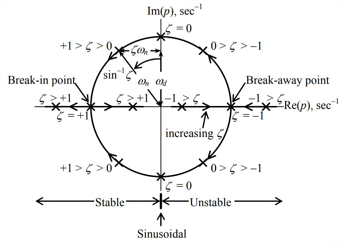
For \(-1>\zeta\), the two real roots, Equation \(\ref{eqn:16.48a}\), are in the right (“east”) half of the \(p\)-plane, on the \(\operatorname{Re}(p)\) axis; the type of time response associated with these roots is monotonically growing exponential, an instability. At \(\zeta=-1\), these two real roots come together with value \(+\omega_{n}\); this is called a “break-away” point because, for the slightest increase in \(\zeta\) above −1, the roots separate into complex conjugates, Equation \(\ref{eqn:16.48b}\), one root headed directly “northward” and the other directly “southward.” The type of response associated with complex conjugate roots that are in the right half-plane off the \(\operatorname{Re}(p)\) axis is oscillation modulated by a growing exponential envelope, an instability. For \(+1>\zeta>-1\), the loci of roots form a perfect circle of radius \(\omega_{n}\) and centered on the origin: \(x^{2}+y^{2}=\left(-\zeta \omega_{n}\right)^{2}+\left(\pm \omega_{d}\right)^{2}=\omega_{n}^{2}\). The roots for \(\zeta=0\) are imaginary, \(p_{1,2}=\pm j \omega_{n}\), for which the time response has pure, undamped sinusoidal form. For \(+1>\zeta>0\), the complex conjugate roots are in the left (“west”) half-plane off the \(\operatorname{Re}(p)\) axis; the type of time response associated with these complex conjugate roots is oscillation modulated by a decaying exponential envelope, which is stable response. As increasing \(\zeta\) approaches the value +1, the two complex roots come together and become real, with value \(-\omega_{n}\), at the “break-in” point. Finally, as \(\zeta\) increases above +1, one real root heads farther westward on the \(\operatorname{Re}(p)\) axis, and the other creeps eastward toward the origin; the type of time response associated with these real roots in the left half-plane is monotonically decaying exponential, which is stable response.

Keep in mind that both monotonic-exponential response and oscillatory response are bounded by the exponential envelope \(e^{\operatorname{Re}(p) t}\). If \(\operatorname{Re}(p)<0\), in the left half-plane, then we define, as in Equation 9.4.3, the 2^nd order time constant, \(\tau_{2} \equiv-1 / \operatorname{Re}(p)>0\), so that the decaying exponential envelope is \(e^{-t / \tau_{2}}\); \(\tau_{2}\) is the time for the stable exponential envelope to decrease by the factor \(e^{-1}\). The degree of positive stability associated with a particular stable root increases as \(\operatorname{Re}(p)\) becomes progressively more negative and \(\tau_{2}\) becomes progressively smaller. In other words, the farther westward from the origin that a pole is located, the greater is the degree of positive stability associated with that pole. On the other hand, if \(\operatorname{Re}(p)>0\), in the right half-plane, then \(+1 / \operatorname{Re}(p)\) is the time for the unstable exponential envelope to increase by the factor \(e^{+1}\). The degree of instability associated with a particular unstable root increases progressively as \(\operatorname{Re}(p)\) becomes progressively more positive; in other words, the instability worsens as the unstable pole moves farther eastward from the origin. Although these observations are made in the context of Figure \(\PageIndex{1}\), they are equally applicable to the loci of roots of any LTI system having any order.

Note on Figure \(\PageIndex{1}\) the construction of a right triangle consisting of horizontal leg \(\zeta \omega_{n}\), vertical leg \(\omega_{d}\), and hypotenuse \(\omega_{n}\), which extends from the origin to a complex pole \(p\). This right triangle is based on the definition \(\omega_{d}^{2}=\omega_{n}^{2}\left(1-\zeta^{2}\right)=\omega_{n}^{2}-\left(\zeta \omega_{n}\right)^{2}\), which is valid for \(|\zeta|<1\). Thus, the frequency of vibration (in rad/s) associated with this particular complex pole is the vertical leg \(\omega_{d}\) along the \(\operatorname{Im}(p)\) axis. Further, the horizontal leg \(\zeta \omega_{n}\) (if in the left half-plane) determines the time constant, \(\tau_{2}=1 / \zeta \omega_{n}\) (in s). Finally, the value of damping ratio \(\zeta\) is the sine of the angle labeled on Figure \(\PageIndex{1}\) between the \(\operatorname{Im}(p)\) axis and hypotenuse \(\omega_{n}\); for a stable pole \(p\) in the left half-plane, as drawn on Figure \(\PageIndex{1}\), \(\zeta\) is positive; for an unstable pole \(p\) in the right half-plane, \(\zeta\) would be negative. Although this derivation is based on \(\PageIndex{1}\), these methods derived for determining the frequency \(\omega_{d}\), time constant \(\tau_{2}\), and damping ratio \(\zeta\) associated with a particular complex pole are applicable to the loci of roots of any LTI system.

Figure \(\PageIndex{1}\) shows the loci of roots of a 2^nd order system as generalized damping, represented by \(\zeta\), varies. Next, let us consider the loci of roots for a 2^nd order system as generalized stiffness varies. Rather than using the symbols \(\zeta\) and \(\omega_{n}\), it is better for this task to revert back to the notation of Section 9.1 representing a generalized mass-damperspring system. Accordingly, we have Equation 7.1.3, \(\omega_{n}^{2}=k / m\), and from Equation 9.1.6, \(\omega_{n}^{2}=k / m\). In these definitions, we specify that \(k\) represents a generalized stiffness, which will vary, and that \(c\) and \(m\) represent, respectively, generalized damping and generalized inertia, which are considered positive constants and will remain fixed while \(k\) varies. For convenience, let us use the following simplified notation:

\[\omega_{n}^{2}=k / m \equiv K \quad \text { and } \quad \zeta \omega_{n}=c /(2 m) \equiv C\label{eqn:16.49} \]

Therefore, for the case \(c / 2 m \geq k / m\), we re-write the real roots Equation \(\ref{eqn:16.48a}\) as

\[p_{1,2}=-\zeta \omega_{n} \pm \sqrt{\left(\zeta \omega_{n}\right)^{2}-\omega_{n}^{2}}=-C \pm \sqrt{C^{2}-K}\label{eqn:16.50a} \]

For \(k / m \geq c / 2 m\), the complex conjugate roots Equation \(\ref{eqn:16.48b}\) are

\[p_{1,2}=-\zeta \omega_{n} \pm j \sqrt{\omega_{n}^{2}-\left(\zeta \omega_{n}\right)^{2}}=-C \pm j \sqrt{K-C^{2}}\label{eqn: 16.50b} \]

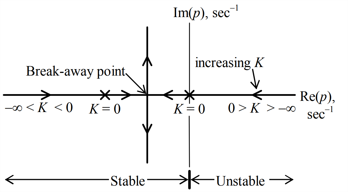
Figure \(\PageIndex{2}\) is an incomplete graph of loci of roots Equations \(\ref{eqn:16.50a}\) and \(\ref{eqn:16.50b}\) as \(K\) varies with \(C > 0\) fixed. (Homework Problem 16.3 is an exercise for completing the task.) Partial annotation shows the locations of the two real poles for \(K=0\). Note, in particular, that for \(K < 0\) one real locus is entirely in the right half-plane. The type of time response associated with this locus is monotonically growing exponential, an instability. (Of course, Routh also shows that the system is unstable for \(K < 0\) and \(C > 0\), since then coefficients of the characteristic equation have different signs.) The passive mechanical springs with which we are familiar always have positive stiffness, so it might appear that this type of instability is purely academic, without any practical significance. Such is not the case. Recall that, in the present discussion, \(k\) (and therefore \(K\) also) represents generalized or total stiffness, not just mechanical stiffness. An elastically restrained airfoil within an air stream is one practical engineering system for which the total stiffness is not necessarily positive. As shown in the discussion accompanying Equation 11.3.8, the total mechanical plus aerodynamic stiffness of this system can become zero or even negative at high airspeeds; the resulting unbounded pitching of the airfoil, called aeroelastic divergence, is an important example of the type of instability represented in Figure \(\PageIndex{2}\) for \(K < 0\).

Figure \(\PageIndex{2}\): Loci roots of \(p^{2}+2 C p+K=0\) as \(K\) varies from \(-\infty\) to greater than \(C^2\), with \(C > 0\) held constant. (Copyright; author via source)

Developing loci-of-roots graphs Figure \(\PageIndex{1}\) and \(\PageIndex{2}\) for 2^nd order systems is relatively simple, but useful as an instructive introduction to this type of stability analysis. In the next section, we will consider the more demanding task of determining loci of roots for systems of higher order.