16.3: Routh’s Stability Criteria

We denote the transfer function of an \(n\)^th order LTI system as \(T F(s)=\frac{\operatorname{Num}(s)}{\operatorname{Den}(s)}\), in which \(\operatorname{Den}(s)\) is an \(n\)^th degree polynomial in \(s\). As derived in Section 16.1, the system is stable or unstable depending upon the signs of the roots of the characteristic equation,

\[\operatorname{Den}(p)=a_{1} p^{n}+a_{2} p^{n-1}+\cdots+a_{n} p+a_{n+1}=0\label{eqn:16.33} \]

For positive stability, we must have \(\operatorname{Re}\left(p_{k}\right)<0\) for all roots, \(k=1,2, \ldots, n\). The roots are dependent upon the polynomial coefficients \(a_{1}, a_{2}, \ldots, a_{n}, a_{n+1}\), so it would seem that the state of stability could be determined directly from these coefficients, without the necessity of calculating the roots. This is indeed the case, and the conditions that these coefficients must satisfy for positive stability are known as Routh’s stability criteria (after Edward John Routh, 1831-1907, English mathematician, physicist, and educator, who developed the systematic framework). These quantitative criteria can be written for a system of any order \(n\), but they become progressively more complicated as \(n\) increases. For that reason, we examine in this section only the criteria for 1^st, 2^nd, and 3^rd order systems; Routh’s criteria for 4^th order systems are presented in homework Problem 16.9(c).

The first requirement for a system of any order, for the system to be positively stable, is that all coefficients of characteristic Equation \(\ref{eqn:16.33}\) be non-zero and have the same sign. This is a necessary condition but, for \(n > 2\), not a sufficient condition for stability. Consider the simplest case, any 1^st order system:

\[\operatorname{Den}(p)=a_{1} p+a_{2}=0 \Rightarrow p=-\frac{a_{2}}{a_{1}}\label{eqn:16.34} \]

It is clear that \(p<0\) if \(a_{1}\) and \(a_{2}\) are both non-zero and of the same polarity, so no other condition is required for stability. Consider next any 2^nd order system:

\[\operatorname{Den}(p)=a_{1} p^{2}+a_{2} p+a_{3}=0\label{eqn:16.35} \]

The quadratic formula gives the following roots of Equation \(\ref{eqn:16.35}\):

\[p_{1,2}=-\frac{a_{2}}{2 a_{1}} \pm \sqrt{\left(\frac{a_{2}}{2 a_{1}}\right)^{2}-\frac{a_{3}}{a_{1}}}\label{eqn:16.36} \]

Careful study of Equation \(\ref{eqn:16.36}\) shows that these roots have negative real parts only if \(a_{1}\), \(a_{2}\) and \(a_{3}\) all are non-zero and have the same sign. Therefore, for the 2^nd order system, the requirement that all three polynomial coefficients be non-zero and have the same sign is a sufficient as well as necessary condition for stability. Note that \(a_{2} = 0\) means the system has zero damping; if, in addition, \(a_{1}\) and \(a_{3}\) have the same sign, then the free-vibration response of the system is pure sinusoidal oscillation (at the natural frequency) with constant amplitude. In this case, the system is not unstable, since the response is bounded, but it is also not exponentially stable; the response does not decay away to a static equilibrium state.

Finally, let us consider the more challenging 3^rd order system:

\[\operatorname{Den}(p)=a_{1} p^{3}+a_{2} p^{2}+a_{3} p+a_{4}=0\label{eqn:16.37} \]

For the system to be stable, \(a_{1}\), \(a_{2}\), \(a_{3}\) and \(a_{4}\) all must be non-zero and have the same sign. The other requirement for positive stability of a 3^rd order system establishes upper and lower bounds on the product \(a_{1} \times a_{4}\):

\[a_{2} \times a_{3}>a_{1} \times a_{4}>0\label{eqn:16.38} \]

The derivation of these two Routh criteria for stability of a 3^rd order system is relatively simple, but more lengthy than necessary for our study; it is presented clearly by Cannon, 1967, pages 406-409.

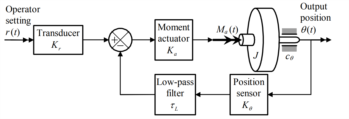
Let us evaluate Routh’s stability criteria applied to the 3^rd order system depicted on Figure \(\PageIndex{1}\). It is similar to the system of Section 14.3 for output-position-feedback control of rotor position, but there are two additions to that system. First, there is bearing friction that produces a passive rotational moment, \(-c_{\theta} \dot{\theta}\), with \(c_{\theta}\) being the viscous damping constant. Second, there is, in the feedback branch downstream of the position sensor, an electrical 1^st order low-pass filter with time constant \(\tau_{L}\). The filtering of sensor voltage signals in this fashion is very common in practice. The usual purpose for low-pass filtering is to cut out high-frequency electrical components from the sensor signal. Such unwanted components might arise from the electronics in a “noisy” sensor, from stray electromagnetic fields and/or improperly shielded electrical cables, and even from extraneous mechanical vibrations. So the amplitude-reduction function of a low-pass filter is almost always beneficial to control-system functioning. However, a low-pass filter also changes the phase of sensor signals, as well as reducing the amplitude of high-frequency-noise, as shown on Figure 4.3.2.

Figure \(\PageIndex{1}\): Functional diagram of a rotor position-feedback control system with a 1^st order low-pass filter in the feedback branch. (Copyright; author via source)

Phase shifts can produce adverse effects on control systems, including reduction of control effectiveness and degradation of system stability, even to instability. From Figure 4.3.2, we see that the extreme phase shift introduced by a 1^st order low-pass filter is −90°, and we can think of this as “almost changing the sign” of the signal that goes through the filter. According to Routh’s criteria, the change of a sign can produce instability. (The effect on stability would be even more dramatic if there were a 2^nd order, rather than 1^st order, low-pass filter in the feedback branch, Figure 10.2.1 with \(\zeta>\sim 0.5\); the extreme phase shift produced by a 2^nd order filter is −180°, which is a complete sign change in the signal that goes through the filter. See homework Problem 16.5.)

The ODE of motion for the damped rotor comes from Equation 3.3.2: \(J \dot{p}+c_{\theta} p= J \ddot{\theta}+c_{\theta} \dot{\theta}=M_{a}(t)\). With the notation \(L[\theta(t)] \equiv \Theta(s)\), the Laplace transform for zero ICs of the ODE of motion is \(\left(J s^{2}+c_{\theta} s\right) \Theta(s)=L\left[M_{a}(t)\right]\), so that the transfer function of the basic damped-rotor plant is

\[\frac{\Theta(s)}{L\left[M_{a}(t)\right]}=\frac{1}{J s^{2}+c_{\theta} s}\label{eqn:16.39} \]

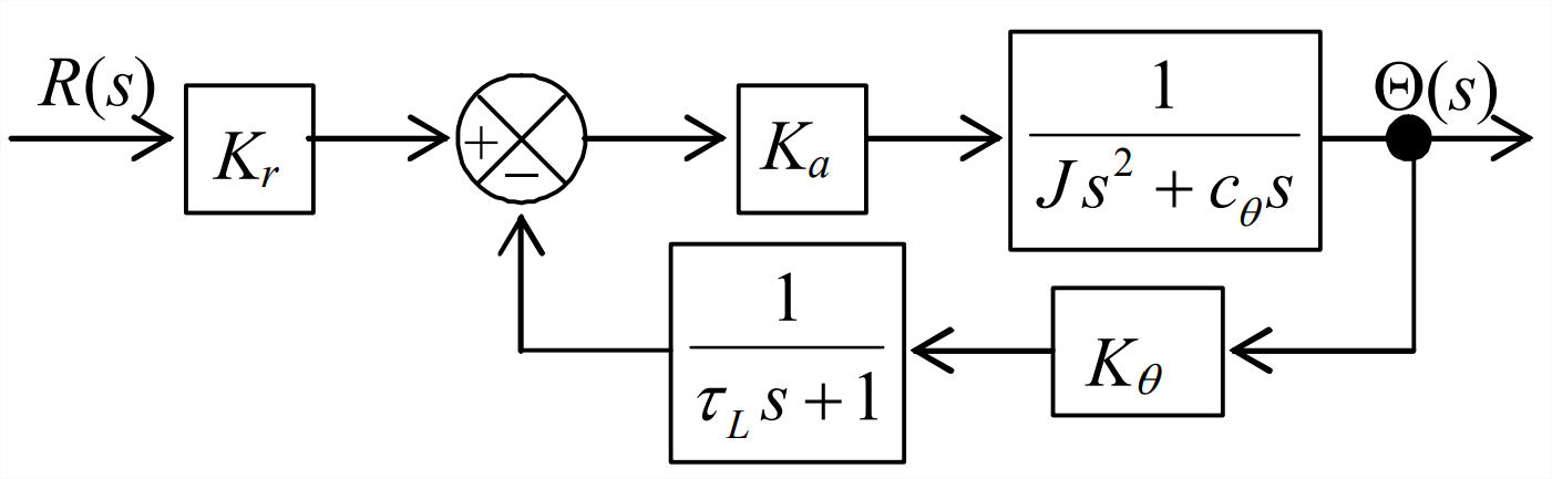
With plant transfer function Equation \(\ref{eqn:16.39}\) and low-pass-filter transfer function Equation 13.1.3, Figure \(\PageIndex{2}\) is the Laplace block diagram for the system of Figure \(\PageIndex{1}\). The branch transfer functions for the loop in Figure \(\PageIndex{1}\) are \(G(s)=\frac{K_{a}}{J s^{2}+c_{\theta} s}\) and \(H(s)=\frac{K_{\theta}}{\tau_{L} s+1}\). Hence, with use of Equation 14.4.6, we find the following closed-loop transfer function:

\[\frac{\Theta(s)}{R(s)}=K_{r} \times \frac{N_{G} D_{H}}{D_{G} D_{H}+N_{G} N_{H}}=K_{r} \times \frac{K_{a}\left(\tau_{L} s+1\right)}{\left(J s^{2}+c_{\theta} s\right)\left(\tau_{L} s+1\right)+K_{a} K_{\theta}} \nonumber \]

Figure \(\PageIndex{2}\): Laplace block diagram of positionfeedback control system with low-pass filtering. (Copyright; author via source)

Algebraic manipulation of this transfer function casts it into the following more useful forms:

\[\frac{\Theta(s)}{R(s)}=\frac{K_{r} K_{a}}{J} \frac{s+1 / \tau_{L}}{s\left(s+\frac{c_{\theta}}{J}\right)\left(s+\frac{1}{\tau_{L}}\right)+\frac{K_{a} K_{\theta}}{J \tau_{L}}}=\frac{K_{r} K_{a}}{J} \frac{s+1 / \tau_{L}}{s^{3}+\left(\frac{1}{\tau_{L}}+\frac{c_{\theta}}{J}\right) s^{2}+\frac{c_{\theta}}{J} \frac{1}{\tau_{L}} s+\frac{K_{a} K_{\theta}}{J \tau_{L}}}\label{eqn:16.40} \]

The two final algebraic forms of Equation \(\ref{eqn:16.40}\) are intended to expedite both evaluation by Routh’s criteria next and by a more general analysis of stability in Section 16.4.

From transfer function Equation \(\ref{eqn:16.40}\) are intended to expedite both evaluation by Routh’s criteria next and by a more general analysis of stability in Section , we find the characteristic equation:

\[\operatorname{Den}(p) \equiv a_{1} p^{3}+a_{2} p^{2}+a_{3} p+a_{4}=p^{3}+\left(\frac{1}{\tau_{L}}+\frac{c_{\theta}}{J}\right) p^{2}+\frac{c_{\theta}}{J} \frac{1}{\tau_{L}} p+\frac{K_{a} K_{\theta}}{J \tau_{L}}=0\label{eqn:16.41} \]

Routh’s first set of criteria for positive stability requires that all polynomial coefficients be non-zero and of the same sign. Since \(a_1 = 1\), the following inequalities are necessary but not sufficient conditions for positive stability:

\[a_{2}=\frac{1}{\tau_{L}}+\frac{c_{\theta}}{J}>0, \quad a_{3}=\frac{c_{\theta}}{J} \frac{1}{\tau_{L}}>0, \text { and } \quad a_{4}=\frac{K_{a} K_{\theta}}{J \tau_{L}}>0\label{eqn:16.42} \]

Rotational inertia \(J\) and filter time constant \(\tau_{L}\) should always be positive physical constants, so Equations \(\ref{eqn:16.42}\) require for positive stability that damping constant \(c_{\theta}\) must be positive, and that the product of sensitivities \(K_{a} K_{\theta}\) must be positive. Routh’s final requirement for positive stability of a 3^rd order system is Equation \(\ref{eqn:16.38}\):

\[a_{2} \times a_{3}>a_{1} \times a_{4}>0 \Rightarrow\left(\frac{1}{\tau_{L}}+\frac{c_{\theta}}{J}\right) \frac{c_{\theta}}{J} \frac{1}{\tau_{L}}>\frac{K_{a} K_{\theta}}{J \tau_{L}}>0 \Rightarrow\left(\frac{1}{\tau_{L}}+\frac{c_{\theta}}{J}\right) \frac{c_{\theta}}{J}>\frac{K_{a} K_{\theta}}{J}>0\label{eqn:16.43a} \]

The common factor \(1 / \tau_{L}\) was removed to produce the final form of Equation \(\ref{eqn:16.43a}\).

Let us suppose that parameters \(J\), \(c_{\theta}\), and \(\tau_{L}\) are positive and fixed, but that the positive product of sensitivities \(K_{a} K_{\theta}\) is a control gain which we have the ability to vary in order to modify the performance and/or stability of the control system. It will be convenient for continued analysis to define a special symbol that denotes the varying fraction in Equation \(\ref{eqn:16.43a}\) and to express the stability requirement in terms of that symbol:

\[\frac{K_{a} K_{\theta}}{J} \equiv \Lambda \Rightarrow\left(\frac{1}{\tau_{L}}+\frac{c_{\theta}}{J}\right) \frac{c_{\theta}}{J}>\Lambda>0\label{eqn:16.43b} \]

Equation \(\ref{eqn:16.43b}\) establishes upper and lower stability boundaries for \(K_{a} K_{\theta} / J \equiv \Lambda\). To illustrate, let us express the stability criterion numerically for some plausible system values. Suppose that the circular break frequency of the low-pass filter is \(\omega_{b} \equiv 1 / \tau_{L}= 300\) rad/s, corresponding to cyclic break frequency \(f_{b}=\omega_{b} / 2 \pi=47.75\) Hz, a realistic value for a low-pass filter used in the control of a mechanical system. Suppose also that the plant parameters have values such that \(c_{\theta} / J=100\) s^-1. Substituting these constants into Equation \(\ref{eqn:16.43b}\) gives the criterion: 40,000 s⁻² \(>\Lambda>0\) for positive stability.

To test the correctness of Routh’s criteria, let us calculate with MATLAB some responses of this system to the initial condition \(\theta(0) \equiv \theta_{0}=0.1\) radian, with all other ICs zero and with zero input, \(r(t)=0\). Let us find the IC response for these three cases:

Case I \(\Lambda_{\mathrm{I}}=0.75 \times\left(\frac{1}{\tau_{L}}+\frac{c_{\theta}}{J}\right) \frac{c_{\theta}}{J}=30,000\) s⁻²; this should give stable response.

Case II \(\Lambda_{\mathrm{II}} \equiv 1.00 \times\left(\frac{1}{\tau_{L}}+\frac{c_{\theta}}{J}\right) \frac{c_{\theta}}{J}=40,000\) s^-2, the upper boundary of stability; but \(\Lambda\) is supposed to be less than 40,000 s⁻² for stability (not equal to it), so what will be the nature of this response?

Case III \(\Lambda_{\mathrm{III}}=1.25 \times\left(\frac{1}{\tau_{L}}+\frac{c_{\theta}}{J}\right) \frac{c_{\theta}}{J}=50,000\) s⁻²; this should give unstable response.

To solve for IC responses of this system, we adapt Equation 16.1.2 to this problem. A little algebra leads us from Equation 16.1.2 to the following transform of the IC response:

\[\Theta(s)=\frac{\theta_{0}\left(a_{1} s^{2}+a_{2} s+a_{3}\right)}{a_{1} s^{3}+a_{2} s^{2}+a_{3} s+a_{4}}\label{eqn:16.44} \]

The \(a_{k}\) constants in Equation \(\ref{eqn:16.44}\) are defined in Equation \(\ref{eqn:16.42}\), and the numerical parameters are given in the paragraph following Equation \(\ref{eqn:16.43b}\). For the numerical values of Cases I, II, and III described above, the partial-fraction expansion of Equation \(\ref{eqn:16.44}\) has the form

\[\Theta(s)=\sum_{k=1}^{3} \frac{C_{k}}{s-p_{k}}=\frac{C_{1}}{s-p_{1}}+\frac{C_{2}}{s-p_{2}}+\frac{\overline{C_{2}}}{s-\overline{p_{2}}}\label{eqn:16.45} \]

in which residue \(C_1\) and pole \(p_1\) are real constants, with \(p_1\) negative for all three cases, and residue \(C_2\) and pole \(p_{2} \equiv \sigma_{2}+j \omega_{2}\) are complex constants. Therefore, from Equations 16.1.9 and 16.1.12, the time response has the form

\[\theta(t)=C_{1} e^{p_{1} t}+2\left|C_{2}\right| e^{\sigma_{2} t} \cos \left(\omega_{2} t+\angle C_{2}\right)\label{eqn:16.46} \]

The MATLAB script M-file below computes the constants of transform Equation \(\ref{eqn:16.45}\), using MATLAB’s residue operation (see homework Problem 2.15), and it computes and plots time response Equation \(\ref{eqn:16.46}\).

%MATLABdemo162.m

%Stability of a damped rotor with low-pass-filtered position feedback

%Excitation with initial position

wb=300;covrJ=100;a2=wb+covrJ;a3=wb*covrJ;Lmub=a2*covrJ;

th0=0.1;t=0:0.0004:0.16;format short e,figure,hold

Lm=[0.75 1 1.25]*Lmub;

for nc=1:3;

a4=Lm(nc)*wb;

Num=th0*[1 a2 a3];Den=[1 a2 a3 a4];[C,p,k]=residue(Num,Den);

disp('Case #, Lambda ='),disp([nc Lm(nc)])

disp('Poles p ='),disp(p.'),disp('Residues C ='),disp(C.')

sig=real(p(2));wd=imag(p(2));abC=abs(C(2));anC=angle(C(2));

th=C(1)*exp(p(1)*t)+2*abC*exp(sig*t).*cos(wd*t+anC);

plot(t,th,'k')

end

grid,xlabel('Time t (sec)'),ylabel('Position \theta (t) (radian)')

title('Response of a 3^r^d order system with different control gains')

The command to execute the M-file, and the resulting alphanumeric output and graphical output (after use of MATLAB’s editing features for annotation and graphical enhancement) follow:

>> MATLABdemo162

Current plot held

Case #, Lambda =

1 30000

Poles p =

-3.8302e+002 -8.4887e+000 +1.5305e+002i -8.4887e+000 -1.5305e+002i

Residues C =

1.4354e-002 4.2823e-002 -2.0336e-002i 4.2823e-002 +2.0336e-002i

Case #, Lambda =

2 40000

Poles p =

-4.0000e+002 -4.3965e-014 +1.7321e+002i -4.3965e-014 -1.7321e+002i

Residues C =

1.5789e-002 4.2105e-002 -1.8232e-002i 4.2105e-002 +1.8232e-002i

Case #, Lambda =

3 50000

Poles p =

-4.1484e+002 7.4222e+000 +1.9001e+002i 7.4222e+000 -1.9001e+002i

Residues C =

1.6864e-002 4.1568e-002 -1.6786e-002i 4.1568e-002 +1.6786e-002i

Figure \(\PageIndex{3}\): Initial-condition response of a rotor output-position-feedback control system with a 1^st order low-pass filter in the feedback branch. (Copyright; author via source)

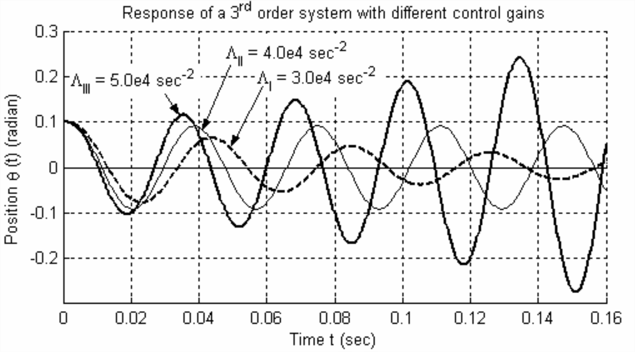
For this system with three poles, at least one pole must be real. For Cases I, II, and III evaluated above, this real pole, \(p_{1}\), turns out to be strongly negative, so it does not contribute to any instability. The second pole, \(p_{2}\), is complex, and the third pole is the conjugate of the second. (The other possibility for a 3^rd order system is that all three poles can be real, but the gains \(\Lambda\) used in this example preclude that.) For gain \(\Lambda_{\mathrm{I}}\), \(\operatorname{Re}\left(p_{2}\right)\) is negative; consequently, the Case I system is positively stable, as predicted by Routh, Equation \(\ref{eqn:16.43b}\). For gain \(\Lambda_{\mathrm{III}}\), \(\operatorname{Re}\left(p_{2}\right)\) is positive; consequently, the Case III system is unstable, also as predicted by Routh. Gain \(\Lambda_{\mathrm{II}}\) is on the upper boundary between positive and negative stability, according to Routh, and the alphanumeric output above shows that \(\operatorname{Re}\left(p_{2}\right)=0\). (The tiny number calculated, −4.4e−14, is non-zero due to roundoff error; comparison of this number with the values of the other poles shows that it is effectively zero.) We see from Figure \(\PageIndex{3}\) that the time response associated with Case II is a pure, undamped sinusoid; the response is bounded, therefore not unstable, but it is not exponentially stable, i.e., it does not decay to zero.

The control system of Figures \(\PageIndex{1}\) and \(\PageIndex{2}\) has two major dynamic sub-systems: the damped rotor with transfer function \(1 /\left[s\left(J s+c_{\theta}\right)\right]\); and the low-pass filter with transfer function \(1 /\left(\tau_{L} s+1\right)\). Each of these passive sub-systems by itself dissipates energy, i.e., acts as an energy sink, and is positively stable. But the complete system is clearly capable of being unstable. The complete system includes an energy source, the moment actuator, and therefore is said to be active. Any system that includes feedback and an energy source is potentially capable of being unstable.

Observe that Routh’s criteria essentially tell us only that a system is stable or unstable, the nature of stability in an absolute sense. They do not tell us the type of response (monotonic-exponential or oscillatory) or the degree of stability (essentially, the magnitudes of the real parts of transfer-function poles), which is also known as relative stability. The method introduced in the next section finds the relative stability.