16.2: Stable and Snstable PD-Controlled-Rotor Systems

In this section, we analyze in detail a specific example of the theory developed in Section 16.1. The situation considered is ideal proportional-derivative (PD) control of position \(\theta(t)\) of a rotor with significant inertia \(J\), as described in Section 15.4 and homework Problem 15.1. The sensitivity of identical input and output-feedback transducers is denoted \(K_{r}=K_{\theta}\), moment actuator sensitivity is \(K_{a}\), and, for the ideal PD controller, proportional gain is \(P\) and derivative time constant is \(\tau_{d}\). The transfer function of this system, from Equations 15.4.3 and 15.4.4, is

\[\frac{\Theta(s)}{R(s)}=\frac{\omega_{n}^{2}\left(\tau_{d} s+1\right)}{s^{2}+2 \zeta \omega_{n} s+\omega_{n}^{2}}\label{eqn:16.14} \]

with 2^nd order-system standard parameters defined as

\[\omega_{n}=\sqrt{\frac{K_{r} K_{a} P}{J}} \text { and } \zeta=\frac{1}{2} \omega_{n} \tau_{d}\label{eqn:15.28} \]

The first useful thing that we can do with transfer function Equation \(\ref{eqn:16.14}\) is infer the system ordinary differential equation (ODE) by inverse Laplace transformation:

\[\left[s^{2}+2 \zeta \omega_{n} s+\omega_{n}^{2}\right] \Theta(s)=\left[\omega_{n}^{2}\left(\tau_{d} s+1\right)\right] R(s) \Rightarrow \ddot{\theta}+2 \zeta \omega_{n} \dot{\theta}+\omega_{n}^{2} \theta=\omega_{n}^{2}\left(\tau_{d} \dot{r}+r\right)\label{eqn:16.15} \]

Recall that the transfer function is based upon zero ICs for the output. But we want to account for ICs now, so let us take the complete Laplace transform of the ODE, including the possibly non-zero ICs, initial rotation rate \(\dot{\theta}(0) \equiv \dot{\theta}_{0}\) and initial position \(\theta(0) \equiv \theta_{0}\):

\[\left[s^{2}+2 \zeta \omega_{n} s+\omega_{n}^{2}\right] \Theta(s)-s \theta_{0}-\dot{\theta}_{0}-2 \zeta \omega_{n} \theta_{0}=\left[\omega_{n}^{2}\left(\tau_{d} s+1\right)\right] R(s)\label{eqn:16.16} \]

The solution of Equation \(\ref{eqn:16.16}\) for the output transform is

\[\Theta(s)=\frac{\theta_{0} s+\left(\dot{\theta}_{0}+2 \zeta \omega_{n} \theta_{0}\right)}{s^{2}+2 \zeta \omega_{n} s+\omega_{n}^{2}}+\frac{\omega_{n}^{2}\left(\tau_{d} s+1\right)}{s^{2}+2 \zeta \omega_{n} s+\omega_{n}^{2}} R(s)\label{eqn:16.17} \]

Compare specific transform solution Equation \(\ref{eqn:16.17}\) with the general form Equation 16.1.5. Next, let us factor the denominator polynomial of the transfer function. It is convenient for this purpose to assume that \(|\zeta|<1\), and to define the positive, real, damped natural frequency as \(\omega_{d}=\omega_{n} \sqrt{1-\zeta^{2}}\). You can easily derive from the quadratic formula (or just substitute in the right-hand side to verify) the factoring:

\[s^{2}+2 \zeta \omega_{n} s+\omega_{n}^{2}=(s-p)(s-\bar{p}), \text { where the complex pole is } p=-\zeta \omega_{n}+j \omega_{d}\label{eqn:16.18} \]

Hence, we re-write transform Equation \(\ref{eqn:16.17}\), and express it in terms of IC-response and forced-response components:

\[\Theta(s)=\frac{\theta_{0} s+\left(\dot{\theta}_{0}+2 \zeta \omega_{n} \theta_{0}\right)}{(s-p)(s-\bar{p})}+\frac{\omega_{n}^{2}\left(\tau_{d} s+1\right)}{(s-p)(s-\bar{p})} R(s) \equiv \Theta_{i c}(s)+\Theta_{f}(s)\label{eqn:16.19} \]

The IC-response term of Equation \(\ref{eqn:16.19}\) is expanded into partial-fraction form:

\[\Theta_{i c}(s) \equiv \frac{\theta_{0} s+\left(\dot{\theta}_{0}+2 \zeta \omega_{n} \theta_{0}\right)}{(s-p)(s-\bar{p})}=\frac{C}{(s-p)}+\frac{\bar{C}}{(s-\bar{p})}\label{eqn:16.20} \]

Using the conventional labor-saving partial-fraction-expansion method of Sections 2.2 and 2.3, and \(p=-\zeta \omega_{n}+j \omega_{d}\) from Equation \(\ref{eqn:16.18}\), and a little algebra, we find the following complex residue of Equation \(\ref{eqn:16.20}\):

\[C=\left[(s-p) \Theta_{i c}(s)\right]_{s=p}=\left[\frac{\theta_{0} p+\left(\dot{\theta}_{0}+2 \zeta \omega_{n} \theta_{0}\right)}{(s-\bar{p})}\right]_{s=p}=\frac{1}{2}\left(\theta_{0}-j \frac{\dot{\theta}_{0}+\zeta \omega_{n} \theta_{0}}{\omega_{d}}\right)\label{eqn:16.21} \]

Hence, substituting Equations \(\ref{eqn:16.18}\) and \(\ref{eqn:16.20}\) into inverse transform Equation 16.1.12 gives the IC-response [with \(C\) given by Equation \(\ref{eqn:16.21}\)]:

\[\theta_{i c}(t)=L^{-1}\left[\Theta_{i c}(s)\right]=2|C| e^{-\zeta \omega_{n} t} \cos \left(\omega_{d} t+\angle C\right)\label{eqn:16.22} \]

Next, let us derive the forced response of this controlled system to a specific, nontrivial input, the ramped exponential pulse \(r(t)=R_{p}(t / \tau) e^{-t / \tau}\), the maximum value of which is \(r_{\max }=r(t=\tau)=R_{p} e^{-1}\). The Laplace transform of this pulse is \(R(s)=\left(R_{p} / \tau\right) /(s+1 / \tau)^{2}\). The transform of the forced response, from Equation \(\ref{eqn:16.19}\), is

\[L\left[\theta_{f}(t)\right]=\frac{\omega_{n}^{2}\left(\tau_{d} s+1\right)}{(s-p)(s-\bar{p})} R(s)=\frac{\omega_{n}^{2}\left(\tau_{d} s+1\right)}{(s-p)(s-\bar{p})} \frac{R_{p} / \tau}{(s+1 / \tau)^{2}}=R_{p} \frac{\omega_{n}^{2}}{\tau} \frac{\tau_{d} s+1}{(s-p)(s-\bar{p})(s+1 / \tau)^{2}}\label{eqn:16.23} \]

The fraction of polynomials in Equation \(\ref{eqn:16.23}\) can be expanded in the following form:

\[L\left[\theta_{f}(t)\right] / R_{p} \frac{\omega_{n}^{2}}{\tau} \equiv F_{f}(s)=\frac{\tau_{d} s+1}{(s-p)(s-\bar{p})(s+1 / \tau)^{2}}=\frac{C R}{s-p}+\frac{\overline{C R}}{s-\bar{p}}+\frac{A}{(s+1 / \tau)^{2}}+\frac{B}{s+1 / \tau}\label{eqn:16.24} \]

\(CR\), \(A\), and \(B\) are constants that we need to find. We have not previously encountered a case of repeated poles such as this. The last two right-hand-side terms in Equation \(\ref{eqn:16.24}\) show the form that a partial-fraction expansion must have for repeated poles (Ogata, 1998, p. 33). We find complex residue \(CR\) using the conventional method:

\[C R=\left[(s-p) F_{f}(s)\right]_{s=p}=\frac{\tau_{d} p+1}{(p-\bar{p})(p+1 / \tau)^{2}}=\frac{\tau_{d} p+1}{j 2 \omega_{d}(p+1 / \tau)^{2}}\label{eqn:16.25} \]

in which \(p=-\zeta \omega_{n}+j \omega_{d}\). To find constants \(A\) and \(B\), it is useful to multiply through Equation \(\ref{eqn:16.24}\) by the denominator factor with repeated poles (Ogata, 1998, p. 33):

\[(s+1 / \tau)^{2} F_{f}(s)=\frac{\tau_{d} s+1}{(s-p)(s-\bar{p})}=(s+1 / \tau)^{2}\left(\frac{C R}{s-p}+\frac{\overline{C R}}{s-\bar{p}}\right)+A+(s+1 / \tau) B\label{eqn:16.26} \]

From Equation \(\ref{eqn:16.26}\), we easily find constant \(A\) using the conventional method:

\[A=\left[(s+1 / \tau)^{2} F_{f}(s)\right]_{s=-1 / \tau}=\frac{-\tau_{d} / \tau+1}{(-1 / \tau-p)(-1 / \tau-\bar{p})}=\frac{1-\tau_{d} / \tau}{(1 / \tau+p)(1 / \tau+\bar{p})}\label{eqn:16.27} \]

Finding constant \(B\) is expedited by first differentiating Equation \(\ref{eqn:16.26}\) with respect to \(s\), so that constant \(B\) stands alone in the last right-hand-side term:

\[\frac{d}{d s}\left[(s+1 / \tau)^{2} F_{f}(s)\right]=\frac{(s-p)(s-\bar{p}) \tau_{d}-\left(\tau_{d} s+1\right)(2 s-p-\bar{p})}{[(s-p)(s-\bar{p})]^{2}} \nonumber \]

\[=\frac{d}{d s}\left[(s+1 / \tau)^{2}\left(\frac{C R}{s-p}+\frac{\overline{C R}}{s-\bar{p}}\right)\right]+B\label{eqn:16.28} \]

\[=2(s+1 / \tau)\left(\frac{C R}{s-p}+\frac{\overline{C R}}{s-\bar{p}}\right)+(s+1 / \tau)^{2} \frac{d}{d s}\left(\frac{C R}{s-p}+\frac{\overline{C R}}{s-\bar{p}}\right)+B \nonumber \]

Hence, we find constant \(B\) by evaluating Equation \(\ref{eqn:16.28}\) at \(s=-1 / \tau\):

\[B=\left\{\frac{(s-p)(s-\bar{p}) \tau_{d}-\left(\tau_{d} s+1\right)(2 s-p-\bar{p})}{[(s-p)(s-\bar{p})]^{2}}\right\}_{s=-1 / z} \nonumber \]

\[=\frac{(1 / \tau+p)(1 / \tau+\bar{p}) \tau_{d}+\left(1-\tau_{d} / \tau\right)(2 / \tau+p+\bar{p})}{[(1 / \tau+p)(1 / \tau+\bar{p})]^{2}}\label{eqn:16.29} \]

Even though \(p\) is complex, \(p=-\zeta \omega_{n}+j \omega_{d}\), the constants \(A\) in Equation \(\ref{eqn:16.27}\) and \(B\) in Equation \(\ref{eqn:16.29}\) turn out to be real. The factors that appear to be complex are: \((1 / \tau+p)(1 / \tau+\bar{p})=\left(1 / \tau-\zeta \omega_{n}+j \omega_{d}\right)\left(1 / \tau-\zeta \omega_{n}-j \omega_{d}\right)=\left(1 / \tau-\zeta \omega_{n}\right)^{2}+\omega_{d}^{2}\), which is real; and \(2 / \tau+p+\bar{p}=2\left(1 / \tau-\zeta \omega_{n}\right)\), which also is real. Thus, the final, more clearly real formulas for constants \(A\) in Equation \(\ref{eqn:16.27}\) and \(B\) in Equation \(\ref{eqn:16.29}\) are

\[A=\frac{1-\tau_{d} / \tau}{\left(1 / \tau-\zeta \omega_{n}\right)^{2}+\omega_{d}^{2}}, B=\frac{\left[\left(1 / \tau-\zeta \omega_{n}\right)^{2}+\omega_{d}^{2}\right] \tau_{d}+2\left(1-\tau_{d} / \tau\right)\left(1 / \tau-\zeta \omega_{n}\right)}{\left[\left(1 / \tau-\zeta \omega_{n}\right)^{2}+\omega_{d}^{2}\right]^{2}}\label{eqn:16.30} \]

With complex residue \(CR\) from Equation \(\ref{eqn:16.25}\), and real constants \(A\) and \(B\) from Equation \(\ref{eqn:16.30}\), the forced-response equation is found from the inverse transform of Equation \(\ref{eqn:16.24}\):

\[\theta_{f}(t)=R_{p} \frac{\omega_{n}^{2}}{\tau} L^{-1}\left[F_{f}(s)\right]=R_{p} \frac{\omega_{n}^{2}}{\tau}\left[2|C R| e^{-\zeta \omega_{n} t} \cos \left(\omega_{d} t+\angle C R\right)+(A t+B) e^{-t / \tau}\right]\label{eqn:16.31} \]

The terms \((A t+B) e^{-t / \tau}\) in Equation \(\ref{eqn:16.31}\) are associated with the poles of the forcing function \(r(t)=R_{p}(t / \tau) e^{-t / \tau}\). Observe that these terms vary in time similarly to \(r(t)\), but that they have no influence over the positive or negative stability of the system. Only the exponential function \(e^{-\zeta \omega_{n} t}\), which is in the term associated with the system (transfer-function) poles, determines the state of system stability.

The complete output equation is the combination of IC-response Equation \(\ref{eqn:16.22}\) and forced-response Equation \(\ref{eqn:16.31}\):

\[\theta(t)=\theta_{i c}(t)+\theta_{f}(t)\label{eqn:16.32} \]

Let us calculate and plot responses for a particular system. The basic parameters are: rotor inertia \(J=0.00256\) lb-s²-inch (the inertia of a small aluminum wheel about four inches in diameter); and product of sensitivities \(K_{r} K_{a}=0.0350\) lb-inch/radian. Let us specify for the closed-loop system: undamped natural frequency \(f_{n}=\omega_{n} /(2 \pi)=1.0\) Hz (so that step-response rise time would be around ¼ s); and damping ratios \(\zeta=+0.12\) for a case of positive stability, and \(\zeta=-0.03\) for a case of instability. The MATLAB Mfile below uses Equation 15.4.4 to calculate the proportional gain \(P=\omega_{n}^{2} J /\left(K_{r} K_{a}\right)=2.888\) and the derivative time constants \(\tau_{d}=2 \zeta / \omega_{n}=0.0382\) s and −0.00955 s listed in the alphanumeric output for the two different cases.

In order to have non-trivial initial conditions, let us specify initial rotation rate \(\dot{\theta}(0) \equiv \dot{\theta}_{0}=-0.29\) rad/s and initial position \(\theta(0) \equiv \theta_{0}=-0.025\) radian. For the ramped-exponential input function \(r(t)=R_{p}(t / \tau) e^{-t / \tau}\), let us specify magnitude \(R_{p}=0.1 \times e\) radian = 0.2718 radian and time constant \(\tau=1.5\) s, so that \(r_{\max }=R_{p} e^{-1}=0.1\) radian at time \(t=1.5\) s. (Most of the input values specified above were chosen by trial and error to produce clear and instructive graphical output.)

A MATLAB script M-file for computing and graphing the response follows:

%MATLABdemo161.m

%Stability of a PD-controlled rotor

%Excitation with initial conditions and a ramped exponential pulse

J=2.56e-3;KrKa=0.035;fn=1;wn=2*pi*fn;P=wn^2*J/KrKa;

disp('P ='),disp(P)

zeta=[0.12 -0.03];

for nc=1:2;

zt=zeta(nc);wd=wn*sqrt(1-zt^2);p=-zt*wn+j*wd;Td=2*zt/wn;

disp('Case #, zeta, Td, p ='),disp([nc zt Td p])

%Initial-condition response

th0=-0.025;dth0=-0.29;

C=(th0-j*(dth0+zt*wn*th0)/wd)/2;abC=abs(C);anC=angle(C);

t=0:.05:10;

thic=2*abC*exp(-zt*wn*t).*cos(wd*t+anC);

%Forced response

Rp=0.1*exp(1);tau=1.5;r=Rp/tau*t.*exp(-t/tau);

CR=(Td*p+1)/(j*2*wd*(p+1/tau)^2);abCR=abs(CR);anCR=angle(CR);

c1=1-Td/tau;c2=1/tau-zt*wn;c3=c2^2+wd^2;A=c1/c3;

B=(c3*Td+2*(1-Td/tau)*c2)/c3^2;

thf=Rp*wn^2/tau*(2*abCR*exp(-zt*wn*t).*cos(wd*t+anCR)+(A*t+B).*exp(-t/tau));

subplot(2,1,nc),plot(t,thic+thf,t,r),grid

end

The command to execute the M-file, and the resulting alphanumeric output and graphical output (after use of MATLAB’s editing features for annotation and graphical enhancement) are:

>> MATLABdemo161

P =

2.8876

Case #, zeta, Td, p =

1.0000 0.1200 0.0382 -0.7540 + 6.2378i

Case #, zeta, Td, p =

2.0000 -0.0300 -0.0095 0.1885 + 6.2804i

Figure \(\PageIndex{1}\): Ramped-exponential input operator setting \(r(t)\) and output rotor positions \(\theta(t)\) for an ideal proportional-derivative (PD) controlled rotor, with two different derivative time constants. (Copyright; author via source)

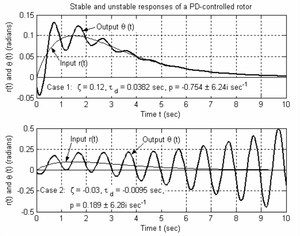
Case 1 of Figure \(\PageIndex{1}\) displays good performance of the PD control system: despite rather adverse initial conditions, the output follows the input nicely, especially after the initial transient response has decayed. In normal engineering practice, derivative time constant \(\tau_{d}\) would probably be set considerably higher than in this academic case, which would suppress the transient oscillation even more quickly and produce even better controlled response.

Case 2, on the other hand, exhibits a serious dynamic instability, which would be unacceptable in normal engineering practice. Note the different \(y\)-axis scales for Cases 1 and 2. In real life, the oscillations would continue to grow exponentially until some mechanical or electrical part would fail (possibly a protective fuse that is designed to fail under excessive load), or some mechanical governor would limit motion, or some electrical component (e.g., an op-amp) would saturate, or until the control system would somehow be disabled intentionally. This example demonstrates that feedback control systems can be dangerous; engineers should design and test any feedback control system with great care in order to make certain that it is positively stable and safe.