1.3: Probability Review

Conditional probabilities and statistical independence

Definition 1.3.1. For any two events \(A\) and \(B\) (with \(\operatorname{Pr}\{B\}>0\)), the conditional probability of \(A\), conditional on \(B\), is defined by

\[\operatorname{Pr}\{A \mid B\}=\operatorname{Pr}\{A B\} / \operatorname{Pr}\{B\}\label{1.12} \]

One visualizes an experiment that has been partly carried out with \(B\) as the result. Then \(\operatorname{Pr}\{A \mid B\}\) can be viewed as the probability of \(A\) normalized to a sample space restricted to event \(B\). Within this restricted sample space, we can view \(B\) as the sample space (i.e., as the set of outcomes that remain possible upon the occurrence of \(B\)) and \(AB\) as an event within this sample space. For a fixed event \(B\), we can visualize mapping each event \(A\) in the original space to event \(AB\) in the restricted space. It is easy to see that the event axioms are still satisfied in this restricted space. Assigning probability \(\operatorname{Pr}\{A \mid B\}\) to each event \(AB\) in the restricted space, it is easy to see that the axioms of probability are satisfied when \(B\) is regarded as the entire sample space. In other words, everything we know about probability can also be applied to such a restricted probability space.

Definition 1.3.2. Two events, \(A\) and \(B\), are statistically independent (or, more briefly, independent) if

\(\operatorname{Pr}\{A B\}=\operatorname{Pr}\{A\} \operatorname{Pr}\{B\}\)

For \(\operatorname{Pr}\{B\}>0\), this is equivalent to \(\operatorname{Pr}\{A \mid B\}=\operatorname{Pr}\{A\}\). This latter form corresponds to our intuitive view of independence, since it says that the observation of \(B\) does not change the probability of \(A\). Such intuitive statements about “observation” and “occurrence” are helpful in reasoning probabilistically, but sometimes cause confusion. For example, Bayes law, in the form \(\operatorname{Pr}\{A \mid B\} \operatorname{Pr}\{B\}=\operatorname{Pr}\{B \mid A\} \operatorname{Pr}\{A\}\), is an immediate consequence of the definition of conditional probability in (1.12). However, if we can only interpret \(\operatorname{Pr}\{A \mid B\}\) when \(B\) is ‘observed’ or occurs ‘before’ \(A\), then we cannot interpret \(\operatorname{Pr}\{B \mid A\}\) and \(\operatorname{Pr}\{A \mid B\}\) together. This caused immense confusion in probabilistic arguments before the axiomatic B} theory was developed.

The notion of independence is of vital importance in defining, and reasoning about, probability models. We will see many examples where very complex systems become very simple, both in terms of intuition and analysis, when appropriate quantities are modeled as statistically independent. An example will be given in the next subsection where repeated independent experiments are used to understand arguments about relative frequencies.

Often, when the assumption of independence turns out to be oversimplified, it is reasonable to assume conditional independence, where \(A\) and \(B\) are said to be conditionally independent given \(C\) if \(\operatorname{Pr}\{A B \mid C\}=\operatorname{Pr}\{A \mid C\} \operatorname{Pr}\{B \mid C\}\). Most of the stochastic processes to be studied here are characterized by particular forms of independence or conditional independence.

For more than two events, the definition of statistical independence is a little more complicated

Definition 1.3.3. The events \(A_{1}, \ldots, A_{n}, n>2\) are statistically independent if for each collection \(S\) of two or more of the integers 1 to \(n\).

\[\left.\operatorname{Pr}\left\{\bigcap_{i \in S} A_{i}\right\}\right\}=\prod_{i \in S} \operatorname{Pr}\left\{A_{i}\right\}\label{1.13} \]

This includes the entire collection \(\{1, \ldots, n\}\), so one necessary condition for independence is that

\[\left.\operatorname{Pr}\left\{\bigcap_{i=1}^{n} A_{i}\right\}\right\}=\prod_{i=1}^{n} \operatorname{Pr}\left\{A_{i}\right\}\label{1.14} \]

It might be surprising that \ref{1.14} does not imply (1.13), but the example in Exercise 1.5 will help clarify this. This definition will become clearer (and simpler) when we see how to view independence of events as a special case of independence of random variables.

Repeated idealized experiments

Much of our intuitive understanding of probability comes from the notion of repeating the same idealized experiment many times (i.e., performing multiple trials of the same experiment). However, the axioms of probability contain no explicit recognition of such repetitions. The appropriate way to handle n repetitions of an idealized experiment is through an extended experiment whose sample points are n-tuples of sample points from the original experiment. Such an extended experiment is viewed as n trials of the original experiment. The notion of multiple trials of a given experiment is so common that one sometimes fails to distinguish between the original experiment and an extended experiment with multiple trials of the original experiment.

To be more specific, given an original sample space \(\Omega\), the sample space of an \(n\)-repetition model is the Cartesian product

\[\Omega^{\times n}=\left\{\left(\omega_{1}, \omega_{2}, \ldots, \omega_{n}\right): \omega_{i} \in \Omega \text { for each } i, 1 \leq i \leq n\right\}\label{1.15} \]

i.e., the set of all n-tuples for which each of the n components of the n-tuple is an element of the original sample space \(\Omega\). Since each sample point in the n-repetition model is an n-tuple of points from the original \(\Omega\), it follows that an event in the n-repetition model is n a subset of \(\Omega^{\times n}\), i.e., a collection of n-tuples \(\left(\omega_{1}, \ldots, \omega_{n}\right)\), where each \(\omega_{i}\) is a sample point from \(\Omega\). This class of events in \(\Omega^{\times n}\) should include each event of the form \(\left\{\left(A_{1} A_{2} \cdots A_{n}\right)\right\}\), where \(\left\{\left(A_{1} A_{2} \cdots A_{n}\right)\right\}\) denotes the collection of n-tuples \(\left(\omega_{1}, \ldots, \omega_{n}\right)\) where \(\omega_{i} \in A_{i}\) for \(1 \leq i \leq n\). The set of events (for n-repetitions) mult also be extended to be closed under complementation and countable unions and intersections.

The simplest and most natural way of creating a probability model for this extended sample space and class of events is through the assumption that the n-trials are statistically independent. More precisely, we assume that for each extended event \(\left\{\left(A_{1} A_{2} \cdots A_{n}\right)\right\}\) contained in \(\Omega^{\times n}\), we have

\[\operatorname{Pr}\left\{\left(A_{1} A_{2} \cdots A_{n}\right)\right\}=\prod_{i=1}^{n} \operatorname{Pr}\left\{A_{i}\right\}\label{1.16} \]

where \(\operatorname{Pr}\left\{A_{i}\right\}\) is the probability of event \(A_{i}\) in the original model. Note that since \(\Omega\) can be substituted for any \(A_{i}\) in this formula, the subset condition of \ref{1.13} is automatically satisfied. In other words, for any probability model, there is an extended independent nrepetition model for which the events in each trial are independent of those in the other trials. In what follows, we refer to this as the probability model for n independent identically distributed (IID) trials of a given experiment.

The niceties of how to create this model for n IID arbitrary experiments depend on measure theory, but we simply rely on the existence of such a model and the independence of events in different repetitions. What we have done here is very important conceptually. A probability model for an experiment does not say anything directly about repeated experiments. However, questions about independent repeated experiments can be handled directly within this extended model of n IID repetitions. This can also be extended to a countable number of IID trials.

Random variables

The outcome of a probabilistic experiment often specifies a collection of numerical values such as temperatures, voltages, numbers of arrivals or departures in various time intervals, etc. Each such numerical value varies, depending on the particular outcome of the experiment, and thus can be viewed as a mapping from the set \(\Omega\) of sample points to the set \(\mathbb{R}\) of real numbers (note that \(\mathbb{R}\) does not include \(\pm \infty\). These mappings from sample points to real numbers are called random variables.

Definition 1.3.4. A random variable \((r v)\) is essentially a function \(X\) from the sample space \(\Omega\) of a probability model to the set of real numbers \(\mathbb{R}\). Three modifications are needed to make this precise. First, \(X\) might be undefined or infinite for a subset of \(\Omega\) that has 0 probability.¹² Second, the mapping \(X(\omega)\) must have the property that \(\{\omega \in \Omega: X(\omega) \leq x\}\) is an event¹³ for each \(x \in \mathbb{R}\). Third, every finite set of \(\text { rv's } X_{1}, \ldots, X_{n}\) has the property that \(\left\{\omega: X_{1}(\omega) \leq x_{1}, \ldots, X_{n}(\omega) \leq x_{n}\right\}\) is an event for each \(x_{1} \in \mathbb{R}, \ldots, x_{n} \in \mathbb{R}\).

As with any function, there is often confusion between the function itself, which is called \(X\) in the definition above, and the value \(X(\omega)\) the function takes on for a sample point \(\omega\). This is particularly prevalent with random variables (rv’s) since we intuitively associate a rv with its sample value when an experiment is performed. We try to control that confusion here by using \(X\), \(X(\omega)\), and \(x\), respectively, to refer to the rv, the sample value taken for a given sample point \(\omega\), and a generic sample value.

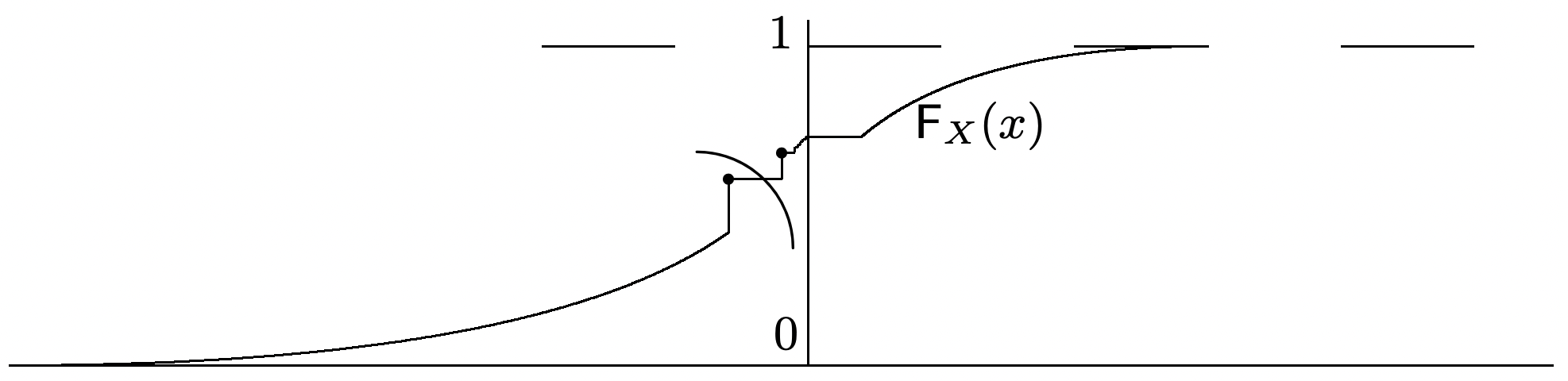
Definition 1.3.5. The distribution function¹⁴ \(\mathrm{F}_{X}(x)\) of a random variable \((r v) X\) is a function, \(\mathbb{R} \rightarrow \mathbb{R}\), defined by \(\mathrm{F}_{X}(x)=\operatorname{Pr}\{\omega \in \Omega: X(\omega) \leq x\}\). The argument \(\omega\) is usually omitted for brevity, so \(\mathrm{F}_{X}(x)=\operatorname{Pr}\{X \leq x\}\).

Note that \(x\) is the argument of \(\mathrm{F}_{X}(x)\) and the subscript \(X\) denotes the particular rv under consideration. As illustrated in Figure 1.1, the distribution function \(\mathrm{F}_{X}(x)\) is nondecreasing with \(x\) and must satisfy the limits \(\lim _{x \rightarrow-\infty} \mathrm{F}_{X}(x)=0\) and \(\lim _{x \rightarrow \infty} \mathrm{F}_{X}(x)=1\). It is not hard to show, from the axioms, that \(\mathrm{F}_{X}(x)\) is continuous from the right (i.e., that for every \(x \in \mathbb{R}\), \(\lim _{k \rightarrow \infty} \mathrm{F}_{X}(x+1 / k)=\mathrm{F}_{X}(x)\).

Figure 1.1: Example of a distribution function for a rv that is neither continuous nor discrete. If \(\mathrm{F}_{X}(x)\) has a discontinuity at some \(x_{o}\), it means that there is a discrete probability at \(x_{o}\) equal to the magnitude of the discontinuity. In this case \(\mathrm{F}_{X}\left(x_{o}\right)\) is given by the height of the upper point at the discontinuity.

Because of the definition of a rv, the set \(\{X \leq x\}\) for any rv \(X\) and any real number \(x\) must be an event, and thus \(\operatorname{Pr}\{X \leq x\}\) must be defined for all real \(x\).

The concept of a rv is often extended to complex random variables (rv’s) and vector rv’s. A complex random variable is a mapping from the sample space to the set of finite complex numbers, and a vector random variable \((rv)\) is a mapping from the sample space to the finite vectors in some finite dimensional vector space. Another extension is that of defective rvs. \(X\) is defective if there is an event of positive probability for which the mapping is either undefined or defined to be either \(+\infty\) or \(-\infty\). When we refer to random variables in this text (without any modifier such as complex, vector, or defective), we explicitly restrict attention to the original definition, i.e., a function from \(\Omega\) to \(\mathbb{R}\).

If \(X\) has only a finite or countable number of possible sample values, say \(x_{1}, x_{2}, \ldots\), the probability \(\operatorname{Pr}\left\{X=x_{i}\right\}\) of each sample value \(x_{i}\) is called the probability mass function (PMF) at \(x_{i}\) and denoted by pX \(\left(x_{i}\right)\); such a random variable is called discrete. The distribution function of a discrete rv is a ‘staircase function,’ staying constant between the possible sample values and having a jump of magnitude pX \(\left(x_{i}\right)\) at each sample value \(x_{i}\). Thus the PMF and the distribution function each specify the other for discrete rv’s.

If the distribution function \(\mathrm{F}_{X}(x)\) of a rv \(X\) has a (finite) derivative at \(x\), the derivative is called the probability density (or the density) of \(X\) at x and denoted by \(\mathrm{f}_{X}(x)\); for suciently small \(\delta\); \(\delta \mathrm{f}_{X}(x)\) then approximates the probability that \(X\) is mapped to a value between \(x\) and \(x+\delta\). If the density exists for all \(x\), the rv is said to be continuous. More generally, if there is a function \(\mathrm{f}_{X}(x)\) such that, for each \(x \in \mathbb{R}\), the distribution function satisfies \(\int_{-infty}^{x} f_{X}(y) d y\), then the rv is said to be continuous and \(\mathrm{f}_{X}\) is the probability density. This generalization allows the density to be discontinuous. In other words, a continuous rv requires a little more than a continuous distribution function and a little less than a continuous density.

Elementary probability courses work primarily with the PMF and the density, since they are convenient for computational exercises. We will often work with the distribution function here. This is partly because it is always defined, partly to avoid saying everything thrice, for discrete, continuous, and other rv’s, and partly because the distribution function is often most important in limiting arguments such as steady-state time-average arguments. For distribution functions, density functions, and PMF’s, the subscript denoting the rv is often omitted if the rv is clear from the context. The same convention is used for complex rv’s and vector rv’s.

Appendix A lists the PMF’s of a number of widely used discrete rv’s and the densities of some equally popular continuous rv’s. The mean, variance and moment generating functions of these variables are also listed for ready reference.

Multiple random variables and conditional probabilities

Often we must deal with multiple random variables (rv’s) in a single probability experiment. If \(X_{1}, X_{2}, \ldots, X_{n}\) are rv’s or the components of a vector rv, their joint distribution function is defined by

\[\mathrm{F}_{X_{1} \cdots X_{n}}\left(x_{1}, x_{2}, \ldots, x_{n}\right)=\operatorname{Pr}\left\{\omega \in \Omega: X_{1}(\omega) \leq x_{1}, X_{2}(\omega) \leq x_{2}, \ldots, X_{n}(\omega) \leq x_{n}\right\} \label{1.17} \]

This definition goes a long way toward explaining why we need the notion of a sample space \(\Omega\) when all we want to talk about is a set of rv’s. The distribution function of a rv fully describes the individual behavior of that rv, but \(\Omega\) and the above mappings are needed to describe how the rv’s interact.

For a vector rv \(\boldsymbol{X}\) with components \(X_{1}, \ldots, X_{n}\), or a complex rv X with real and imaginary parts \(X_{1}, X_{2}\), the distribution function is also defined by (1.17). Note that \(\{X_{1} \leq x_{1}, X_{2} \leq x_2, \dots, X_n \leq x_n\}\) is an event and the corresponding probability is nondecreasing in each argument \(x_{i}\). Also the distribution function of any subset of random variables is obtained by setting the other arguments to \(+\infty\) For example, the distribution of a single rv (called a marginal distribution) is given by

\(\mathrm{F}_{X_{i}}\left(x_{i}\right)=\mathrm{F}_{X_{1} \cdots X_{i-1} X_{i} X_{i+1} \cdots X_{n}}\left(\infty, \ldots, \infty, x_{i}, \infty, \ldots, \infty\right)\)

If the rv’s are all discrete, there is a joint PMF which specifies and is specified by the joint distribution function. It is given by

\(\mathrm{p}_{X_{1} \ldots X_{n}}\left(x_{1}, \ldots, x_{n}\right)=\operatorname{Pr}\left\{X_{1}=x_{1}, \ldots, X_{n}=x_{n}\right\}\)

Similarly, if the joint distribution function is differentiable everywhere, it specifies and is specified by the joint probability density,

\(\mathrm{f}_{X_{1} \ldots X_{n}}\left(x_{1}, \ldots, x_{n}\right)=\frac{\partial^{n} \mathrm{~F}\left(x_{1}, \ldots, x_{n}\right)}{\partial x_{1} \partial x_{2} \cdots \partial x_{n}}\)

Two rv’s, say \(X\) and \(Y\), are statistically independent (or, more briefly, independent) if

\[\mathrm{F}_{X Y}(x, y)=\mathrm{F}_{X}(x) \mathrm{F}_{Y}(y) \quad \text { for each } x \in \mathbb{R}, y \in \mathbb{R}\label{1.18} \]

If \(X\) and \(Y\) are discrete rv’s then the definition of independence in \ref{1.18} is equivalent to the corresponding statement for PMF’s,

\(\mathrm{p}_{X Y}\left(x_{i} y_{j}\right)=\mathrm{p}_{X}\left(x_{i}\right) \mathrm{p}_{Y}\left(y_{j}\right) \quad \text { for each value } x_{i} \text { of } X \text { and } y_{j} \text { of } Y\)

Since \(\left\{X=x_{i}\right\}\) and \(\left\{Y=y_{j}\right\}\) are events, the conditional probability of \(\left\{X=x_{i}\right\}\) conditional on \(\left\{Y=y_{j}\right\}\) (assuming \(\mathrm{p}_{Y}\left(y_{j}\right)>0\)) is given by \ref{1.12} to be

\(\mathrm{p}_{X \mid Y}\left(x_{i} \mid y_{j}\right)=\frac{\mathrm{p}_{X Y}\left(x_{i}, y_{j}\right)}{\mathrm{p}_{Y}\left(y_{j}\right)}\)

If \(\mathrm{p}_{X \mid Y}\left(x_{i} \mid y_{j}\right)=\mathrm{p}_{X}\left(x_{i}\right)\) for all \(i, j\) then it is seen that \(X\) and \(Y\) are independent. This captures the intuitive notion of independence better than \ref{1.18} for discrete rv’s , since it can be viewed as saying that the PMF of \(X\) is not affected by the sample value of \(Y\).

If \(X\) and \(Y\) have a joint density, then \ref{1.18} is equivalent to

\(\mathrm{f}_{X Y}(x, y)=\mathrm{f}_{X}(x) \mathrm{f}_{Y}(y) \quad \text { for each } x \in \mathbb{R}, y \in \mathbb{R}\)

If \(\mathrm{f}_{Y}(y)>0\), the conditional density can be defined as \(\mathrm{f}_{X \mid Y}(x \mid y)=\frac{\mathrm{f}_{X Y}(x, y)}{f_{Y}(y)}\). Then fY \ref{y} statistical independence can be expressed as \(\mathrm{f}_{X \mid Y}(x \mid y)=\mathrm{f}_{X}(x) \quad \text { where } \mathrm{f}_{Y}(y)>0\label{1.19}\)

This captures the intuitive notion of statistical independence for continuous rv’s better than (1.18), but it does not quite say that the density of \(X\), conditional on \(Y=y\) is the same as the marginal density of \(X\). The event \(\{Y=y\}\) has zero probability for a continuous rv, and we cannot condition on events of zero probability. If we look at the derivatives defining these densities, the conditional density looks at the probability that \(\{x \leq X \leq x+\delta\}\) given that \(\{y \leq Y \leq y+\epsilon\}\) in the limit \(\delta, \epsilon \rightarrow 0\). At some level, this is a very technical point and the intuition of conditioning on \(\{Y=y\}\) works very well. Furthermore, problems are often directly modeled in terms of conditional probability densities, so that viewing a conditional density as a limit is less relevant.

More generally the probability of an arbitrary event \(A\) conditional on a given value of a continuous rv \(Y\) is given by

\(\operatorname{Pr}\{A \mid Y=y\}=\lim _{\delta \rightarrow 0} \frac{\operatorname{Pr}\{A, Y \in[y, y+\delta]\}}{\operatorname{Pr}\{Y \in[y, y+\delta]\}}\)

We next generalize the above results about two rv’s to the case of \(n\) rv’s \(\boldsymbol{X}=X_{1}, \ldots, X_{n}\). Statistical independence is then defined by the equation

\[\mathrm{F}_{\boldsymbol{X}}\left(x_{1}, \ldots, x_{n}\right)=\prod_{i=1}^{n} \operatorname{Pr}\left\{X_{i} \leq x_{i}\right\}=\prod_{i=1}^{n} \mathrm{~F}_{X_{i}}\left(x_{i}\right) \quad \text { for all values of } x_{1}, \ldots, x_{n}\label{1.20} \]

In other words, \(X_{1}, \ldots, X_{n}\) are independent if the events \(X_{i} \leq x_{i}\) or \(1 \leq i \leq n\) are independent for all choices of \(x_{1}, \ldots, x_{n}\). If the density or PMF exists, \ref{1.20} is equivalent to a product form for the density or mass function. A set of rv’s is said to be pairwise independent if each pair of rv’s in the set is independent. As shown in Exercise 1.20, pairwise independence does not imply that the entire set is independent.

Independent rv’s are very often also identically distributed, i.e., they all have the same distribution function. These cases arise so often that we abbreviate independent identically distributed by IID. For the IID case \ref{1.20} becomes

\[\mathrm{F}_{X}\left(x_{1}, \ldots, x_{n}\right)=\prod_{i=1}^{n} \mathrm{~F}_{X}\left(x_{i}\right)\label{1.21} \]

Stochastic processes and the Bernoulli process

A stochastic process (or random process¹⁵) is an infinite collection of rv’s, usually indexed by an integer or a real number often interpreted as time.16 Thus each sample point of the probability model maps to an infinite collection of sample values of rv’s. If the index is regarded as time, then each sample point maps to a function of time called a sample path or sample function. These sample paths might vary continuously with time or might vary only at discrete times, and if they vary at discrete times, those times might be deterministic or random.

In many cases, this collection of rv’s comprising the stochastic process is the only thing of interest. In this case the sample points of the probability model can be taken to be the sample paths of the process. Conceptually, then, each event is a collection of sample paths. Often these events are defined in terms of a finite set of rv’s.

As an example of sample paths that vary at only discrete times, we might be concerned with the times at which customers arrive at some facility. These ‘customers’ might be customers entering a store, incoming jobs for a computer system, arriving packets to a communication system, or orders for a merchandising warehouse.

The Bernoulli process is an example of how such customers could be modeled and is perhaps the simplest non-trivial stochastic process. We define this process here and develop a few of its many properties. We will frequently return to it, both to use it as an example and to develop additional properties.

Example 1.3.1. A Bernoulli process is a sequence, \(Y_{1}, Y_{2}, \ldots\), of IID binary random variables.¹⁷ Let \(p=\operatorname{Pr}\left\{Y_{i}=1\right\}\) and \(1-p=\operatorname{Pr}\left\{Y_{i}=0\right\}\). We usually visualize a Bernoulli process as evolving in discrete time with the event \(\left\{Y_{i}=1\right\}\) representing an arriving customer at time \(i\) and \(\left\{Y_{i}=0\right\}\) representing no arrival. Thus at most one arrival occurs at each integer time. We visualize the process as starting at time 0, with the first opportunity for an arrival at time 1.

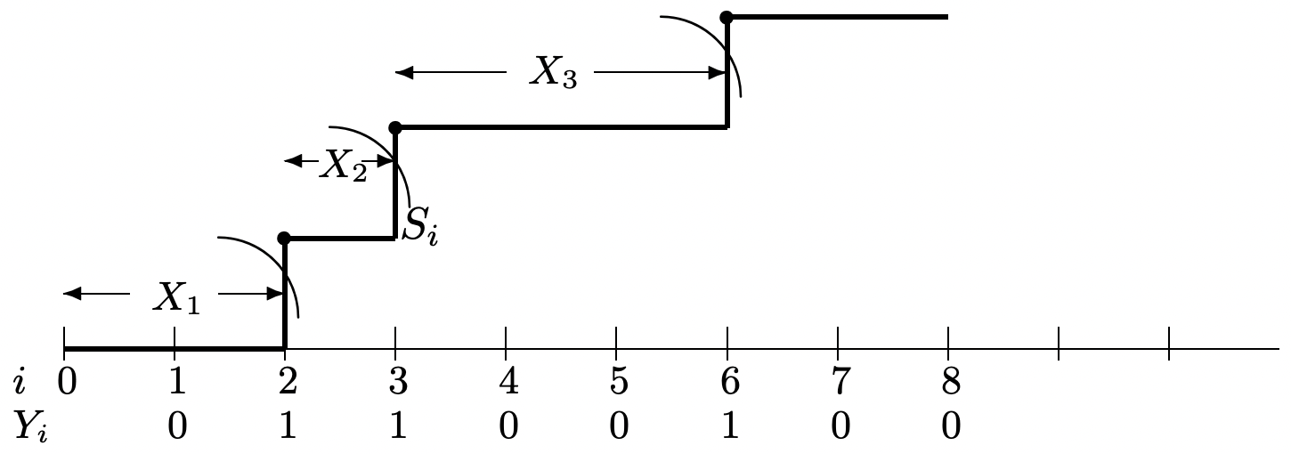
When viewed as arrivals in time, it is interesting to understand something about the intervals between successive arrivals, and about the aggregate number of arrivals up to any given time (see Figure 1.2). These interarrival times and aggregate numbers of arrivals are rv’s that are functions of the underlying sequence \(Y_{1}, Y_{2}, \ldots\),. The topic of rv’s that are defined as functions of other rv’s (i.e., whose sample values are functions of the sample values of the other rv’s) is taken up in more generality in Section 1.3.7, but the interarrival times and aggregate arrivals for Bernoulli processes are so specialized and simple that it is better to treat them from first principles.

First, consider the first interarrival time, \(X_{1}\), which is defined as the time of the first arrival. If \(Y_{1}=1\), then (and only then) \(X_{1}=1\). Thus \(\mathrm{p}_{X_{1}}(1)=p\). Next, \(X_{1}=2\) if and only \(Y_{1}=0\) and \(Y_{2}=1\), so \(\mathrm{p}_{X_{1}}(2)=p q\). Continuing, we see that \(X_{1}\) has the geometric PMF,

\(\mathrm{p}_{X_{1}}(j)=p(1-p)^{j-1}\)

Each subsequent interarrival time \(X_{k}\) can be found in this same way.¹⁸ It has the same geometric PMF and is statistically independent of \(X_{1}, \ldots, X_{k-1}\). Thus the sequence of interarrival times is an IID sequence of geometric rv’s.

It can be seen from Figure 1.2 that a sample path of interarrival times also determines a sample path of the binary arrival rv’s, \(\left\{Y_{i} ; i \geq 1\right\}\). Thus the Bernoulli process can also be characterized as a sequence of IID geometric rv’s.

For our present purposes, the most important rv’s in a Bernoulli process are the partial sums \(S_{n}=\sum_{i=1}^{n} Y_{i}\). Each rv \(S_{n}\) is the number of arrivals up to and includng time \(n\) i.e.,

Figure 1.2: Illustration of a sample path for a Bernoulli process: The sample values of the binary rv’s \(Y_{i}\) are shown below the time instants. The sample value of the aggregate number of arrivals, \(S_{n}=\sum_{i=1}^{n} Y_{i}\), is the illustrated step function, and the interarrival intervals are the intervals between steps.

\(S_{n}\) is simply the sum of \(n\) binary rv’s and thus has the binomial distribution. The PMF \(\mathrm{p}_{S_{n}}(k)\) is the probability that \(k\) out of \(n\) of the \(Y_{i} \text { 's }\) have the value 1. There are \(\left.\left(\begin{array}{l} n \\ k \end{array}\right)\right\}=\frac{n !}{k !(n-k) !}\) arrangements of \(n\) binary numbers with \(k\) 1’s, and each has probability \(p^{k} q^{n-k}\). Thus

\[\mathbf{p}_{S_{n}}(k)=\left(\begin{array}{l} n \\ k \end{array}\right) p^{k} q^{n-k}\label{1.22} \]

We will use the binomial PMF extensively as an example in explaining the laws of large numbers later in this chapter, and will often use it in later chapters as an example of a sum of IID rv’s. For these examples, we need to know how \(\mathrm{p}_{S_{n}}(k)\) behaves asymptotically as \(n \rightarrow \infty\) and \(k \rightarrow \infty\) with \(k / n\) essentially constant. The relative frequency (\ k / n\) will be denoted as \(\tilde{p}\). We make a short digression here to state and develop an approximation to the binomial PMF that makes this asymptotic behavior clear.

Lemma 1.3.1. Let \(\mathrm{p}_{S_{n}}(\tilde{p} n)\) be the PMF of the binomial distribution for an underlying binary PMF \(\mathrm{p}_{Y}(1)=p>0\), \(\mathrm{p}_{Y}(0)=q>0\). Then for each integer \(\tilde{p} n\), \(1 \leq \tilde{p} n \leq n-1\),

\[\left.\left.\mathrm{p}_{S_{n}}(\tilde{p} n)\right)<\sqrt{\frac{\}1}{2 \pi n \tilde{p}(1-\tilde{p})}} \exp [n \phi(p, \tilde{p})]\right\} \text{where} \label{1.23} \]

\[\phi(p, \tilde{p})=\tilde{p} \ln \left(\frac{p}{\tilde{p}}\right)+(1-\tilde{p}) \ln \left(\frac{1-p}{1-\tilde{p}}\right) \leq 0 \label{1.24} \]

Also, \(\phi(p, \tilde{p})<0\) for all \(\tilde{p} \neq p\). Finally, for any \(\epsilon>0\), there is an \(n(\epsilon)\) such that for \(n>n(\epsilon)\),

\[\left.\mathrm{p}_{S_{n}}(\tilde{p} n)>\left(1-\frac{1}{\sqrt{n}}\right) \sqrt{\frac{\}1}{2 \pi n \tilde{p}(1-\tilde{p})}} \exp [n \phi(p, \tilde{p})]\right\} \quad \text { for } \epsilon \leq \tilde{p} \leq 1-\epsilon\label{1.25} \]

Discussion: The parameter \(\tilde{p}=k / n\) is the relative frequency of 1’s in the \(n\)-tuple \(Y_{1}, \ldots, Y_{n}\). For each \(n\), \(\tilde{p}\) on the left of \ref{1.23} is restricted so that \(\tilde{p} n\) is an integer. The lemma then says that \(p_{S_{n}}(\tilde{p} n)\) is upper bounded by an exponentially decreasing function of \(n\) for each \(\tilde{p} \neq p\).

If \(\tilde{p}\) is bounded away from 0 and 1, the ratio of the upper and lower bounds on \(p_{S_{n}}(\tilde{p} n)\) approaches 1 as \(n \rightarrow \infty\). A bound that is asymptotically tight in this way is denoted as

\[\left.\left.\mathrm{p}_{S_{n}}(\tilde{p} n)\right) \sim \sqrt{\frac{\}1}{2 \pi n \tilde{p}(1-\tilde{p})}} \exp [n \phi(p, \tilde{p})]\right\} \quad \text { for } \epsilon<\tilde{p}<1-\epsilon\label{1.26} \]

where the symbol ~ means that the ratio of the left and right side approach 1 as \(n \rightarrow \infty\)

\[\sqrt{2 \pi n}\left(\frac{n}{e}\right)^{n}<n !<\sqrt{2 \pi n}\left(\frac{n}{e}\right)^{n} e^{1 / 12 n}\label{1.27} \]

The ratio \(\sqrt{2 \pi n}(n / e)^{n} / n\)! is monotonically increasing with \(n\) toward the limit 1, and the ratio \(\sqrt{2 \pi n}(n / e)^{n} \exp (1 / 12 n) / n!\) is monotonically decreasing toward 1. The upper bound is more accurate, but the lower bound is simpler and known as the Stirling approximation.

Since \(\sqrt{2 \pi n}(n / e)^{n} / n!\) is increasing in \(n\), we see that \(n ! / k !<\sqrt{n / k} n^{n} k^{-k} e^{-n+k} \text { for } k<n\).

Combining this with \ref{1.27} applied to \(n-k\),

\[\left.\left(\begin{array}{l} n \\ k \end{array}\right)\right\}<\sqrt{\frac{\}n}{2 \pi k(n-k)}} \frac{n^{n}}{k^{k}(n-k)^{n-k}}\label{1.28} \]

Using \ref{1.28} in \ref{1.22} to upper bound \(\mathrm{p}_{S_{n}}(k)\),

\(\mathrm{p}_{S_{n}}(k)<\sqrt{\frac{\}n}{2 \pi k(n-k)}} \frac{p^{k} q^{n-k} n^{n}}{k^{k}(n-k)^{n-k}}\)

Replacing \(k\) by \(\tilde{p} n\), we get \ref{1.23} where \(\phi(p, \tilde{p})\) is given by (1.24). Applying the same argument to the right hand inequality in (1.27),

\[\begin{aligned}
\left(\begin{array}{l}
n \\ k \end{array}\right)^{\}} &>\sqrt{\frac{n}{2 \pi k(n-k)}} \frac{n^{n}}{k^{k}(n-k)^{n-k}} \exp \left(-\frac{1}{12 k}-\frac{1}{12(n-k)}\right)^{\}} \\
&>\sqrt{\frac{n}{2 \pi k(n-k)}} \frac{n^{n}}{k^{k}(n-k)^{n-k}}\left[1-\frac{1}{12 n \tilde{p}(1-\tilde{p})}\right]
\end{aligned}\label{1.29} \]

For \(\epsilon<\tilde{p}<1-\epsilon\), the term in brackets in \ref{1.29} is lower bounded by \(1-1 /(12 n \epsilon(1-\epsilon)\), which is further lower bounded by \(1-1 / \sqrt{n}\) for all suciently large \(n\), establishing (1.25).

Finally, to show that \(\phi(p, \tilde{p}) \leq 0\), with strict inequality for \(\tilde{p} \neq p\), we take the first two derivatives of \(\phi(p, \tilde{p})\) with respect to \(\tilde{p}\).

\(\left.\frac{\partial \phi(p, \tilde{p})}{\partial \tilde{p}}=\ln \left(\frac{p(1-\tilde{p})}{\tilde{p}(1-p)}\right)\right\} \quad \quad \quad \quad \frac{\partial f^{2}(p, \tilde{p})}{\partial \tilde{p}^{2}}=\frac{-1}{\tilde{p}(1-\tilde{p})}\)

Since the second derivative is negative for \(0<\tilde{p}<1\), the maximum of \(\phi(p, \tilde{p})\) with respect to \(\tilde{p}\) is 0, achieved at \(\tilde{p}=p\). Thus \(\phi(p, \tilde{p})<0\) for \(\tilde{p} \neq p\). Furthermore, \(\phi(p, \tilde{p})\) decreases as \(\tilde{p}\) moves in either direction away from \(p\).

Various aspects of this lemma will be discussed later with respect to each of the laws of large numbers.

We have seen that the Bernoulli process can also be characterized as a sequence of IID geometric interarrival intervals. An interesting generalization of this arises by allowing the interarrival intervals to be arbitrary discrete or continuous nonnegative IID rv’s rather than geometric rv’s. These processes are known as renewal processes and are the topic of Chapter 3. Poisson processes are special cases of renewal processes in which the interarrival intervals have an exponential PDF. These are treated in Chapter 2 and have many connections to Bernoulli processes.

Renewal processes are examples of discrete stochastic processes. The distinguishing characteristic of such processes is that interesting things (arrivals, departures, changes of state) occur at discrete instants of time separated by deterministic or random intervals. Discrete stochastic processes are to be distinguished from noise-like stochastic processes in which changes are continuously occurring and the sample paths are continuously varying functions of time. The description of discrete stochastic processes above is not intended to be precise. The various types of stochastic processes developed in subsequent chapters are all discrete in the above sense, however, and we refer to these processes, somewhat loosely, as discrete stochastic processes.

Discrete stochastic processes find wide and diverse applications in operations research, communication, control, computer systems, management science, finance, etc. Paradoxically, we shall spend relatively little of our time discussing these particular applications, and rather develop results and insights about these processes in general. Many examples drawn from the above fields will be discussed, but the examples will be simple, avoiding many of the complications that require a comprehensive understanding of the application area itself.

Expectation

The expected value E [X] of a random variable X is also called the expectation or the mean and is frequently denoted as \(\bar{X}\). Before giving a general definition, we discuss several special cases. First consider nonnegative discrete rv’s. The expected value \(\mathrm{E}[X]\) is then given by

\[\mathrm{E}[X]=\sum_{x} x \mathrm{p}_{X}(x)\label{1.30} \]

If X has a finite number of possible sample values, the above sum must be finite since each sample value must be finite. On the other hand, if X has a countable number of nonnegative sample values, the sum in \ref{1.30} might be either finite or infinite. Example 1.3.2 illustrates a case in which the sum is infinite. The expectation is said to exist only if the sum is finite (i.e., if the sum converges to a real number), and in this case E [X] is given by (1.30). If the sum is infinite, we say that E [X] does not exist, but also say²¹ that E [X] = \(\infty\). In other words, \ref{1.30} can be used in both cases, but E [X] is said to exist only if the sum is finite.

Example 1.3.2. This example will be useful frequently in illustrating rv’s that have an infinite expectation. Let \(N\) be a positive integer-valued rv with the distribution function \(\mathrm{F}_{N}(n)=n /(n+1)\) for each integer \(n \geq 1\). Then \(N\) is clearly a positive rv since \(\mathrm{F}_{N}(0)=0\) and \(\lim _{N \rightarrow \infty} \mathrm{F}_{N}(n)=1\). For each \(n \geq 1\), the PMF is given by

\[\mathrm{p}_{N}(n)=\mathrm{F}_{N}(n)-\mathrm{F}_{N}(n-1)=\frac{n}{n+1}-\frac{n-1}{n}=\frac{1}{n(n+1)}\label{1.31} \]

Since \(\mathrm{p}_{N}(n)\) is a PMF, we see that \(\sum_{n=1}^{\infty} 1 /[n(n+1)]=1\), which is a frequently useful sum. The following equation, however, shows that \(\mathrm{E}[N]\) does not exist and has infinite value.

\(\left.\left.\mathrm{E}[N]=\sum_{n=1}^{\infty} n \mathrm{p}_{N}(n)=\sum_{n=1}^{\infty}\right\}_{n(n+1)}=\sum_{n=1}^{\infty}\right\} \frac{1}{n+1}=\infty\),

where we have used the fact that the harmonic series diverges.

We next derive an alternative expression for the expected value of a nonnegative discrete rv. This new expression is given directly in terms of the distribution function. We then use this new expression as a general definition of expectation which applies to all nonnegative rv’s, whether discrete, continuous, or arbitrary. It contains none of the convergence questions that could cause confusion for arbitrary rv’s or for continuous rv’s with very wild densities.

Figure 1.3: The figure shows the complementary distribution function \(\mathrm{F}_{X}^{c}\) of a nonnegative discrete rv \(X\). For this example, \(X\) takes on four possible values, \(0<a_{1}<a_2<a_3<a_4\). Thus \(\mathrm{F}_{X}^{c}(x)=\operatorname{Pr}\{X>x\}=1\) for \(x<a_{1}\). For \(a_{1} \leq x<a_{2}\), \(\operatorname{Pr}\{X>x\}=1-\mathrm{p}_{X}\left(a_{1}\right)\), and \(\operatorname{Pr}\{X>x\}\) has similar drops as \(x\) reaches \(a_{2}\), \(a_{3}\), and \(a_{4}\). \(\mathrm{E}[X]\), from (1.30), is \(\sum_{i} a_{i} \mathrm{p}_{X}\left(a_{i}\right)\), which is the sum of the rectangles in the figure. This is also the area under the curve \(\mathrm{F}_{X}^{c}(x)\), i.e., \(\int_{0}^{\infty} \mathrm{F}_{X}^{c}(x) d x\). It can be seen that this argument applies to any nonnegative rv, thus verifying (1.32).

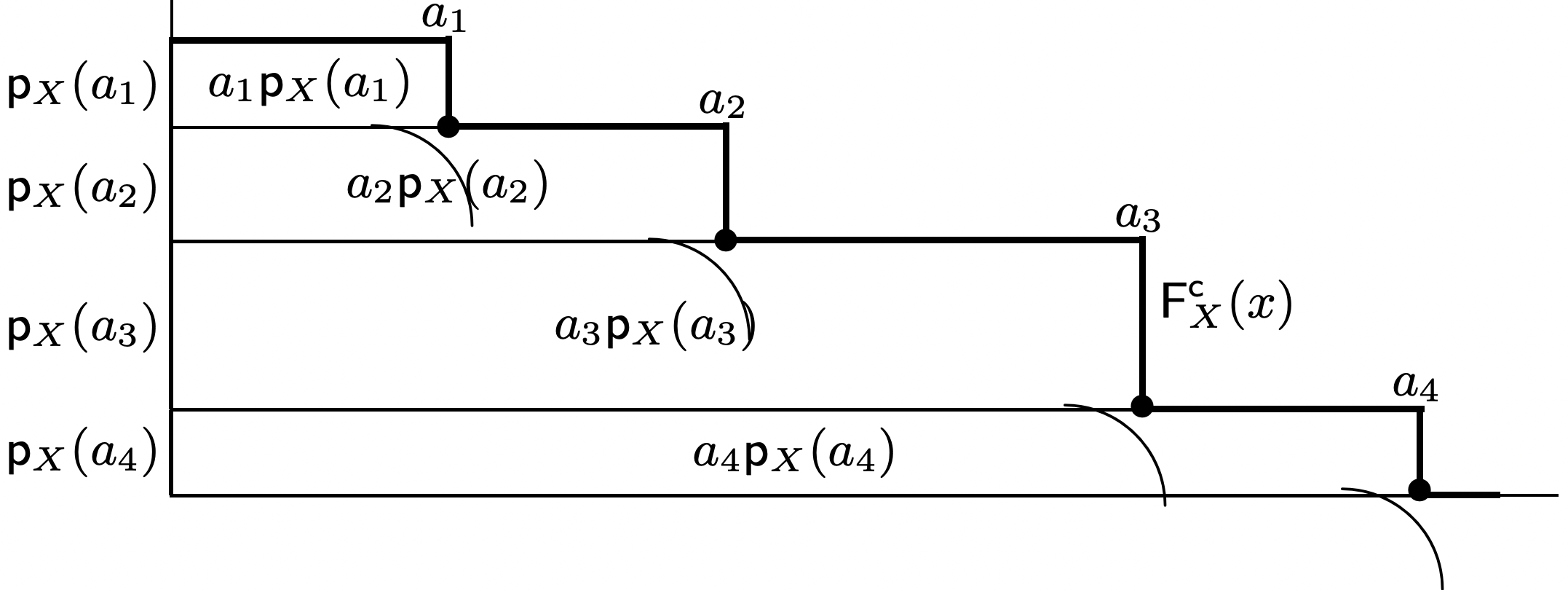
For a nonnegative discrete rv \(X\), Figure 1.3 illustrates that \ref{1.30} is simply the integral of the complementary distribution function, where the complementary distribution function \(\mathrm{F}^{\mathrm{c}}\) of a rv is defined as \(\mathrm{F}_{X}^{\mathrm{c}}(x)=\operatorname{Pr}\{X>x\}=1-\mathrm{F}_{X}(x)\).

\[\mathrm{E}[X]=\int_{0}^{\}\infty} \mathrm{F}_{X}^{c} d x=\int_{0}^{\}\infty} \operatorname{Pr}\{X>x\} d x\label{1.32} \]

Although Figure 1.3 only illustrates the equality of \ref{1.30} and \ref{1.32} for one special case, one easily sees that the argument applies to any nonnegative discrete rv, including those with countably many values, by equating the sum of the indicated rectangles with the integral.

For a continuous nonnegative rv \(X\), the conventional definition of expectation is given by

\[\mathrm{E}[X]=\lim _{b \rightarrow \infty} \int_{0}^{\}b} x \mathrm{f}_{X}(x) d x\label{1.33} \]

Suppose the integral is viewed as a limit of Riemann sums. Each Riemann sum can be viewed as the expectation of a discrete approximation to the continuous rv. The corresponding expectation of the approximation is given by \ref{1.32} using the approximate \(F_{X}\). Thus (1.32), using the true \(\mathrm{F}_{X}\), yields the expected value of \(X\). This can also be seen using integration by parts. There are no mathematical subtleties in integrating an arbitrary nonnegative nonincreasing function, and this integral must have either a finite or infinite limit. This leads us to the following fundamental definition of expectation for nonnegative rv’s:

Definition 1.3.6. The expectation E [X] of a nonnegative rv \(X\) is defined by (1.32). The expectation is said to exist if and only if the integral is finite. Otherwise the expectation is said to not exist and is also said to be infinite.

Next consider rv’s with both positive and negative sample values. If X has a finite number of positive and negative sample values, say \(a_{1}, a_{2}, \ldots, a_{n}\) the expectation E [X] is given by

\[\begin{aligned}
\mathrm{E}[X] &=\sum_{i} a_{i} \mathrm{p}_{X}\left(a_{i}\right) \\
&\left.\left.=\sum_{a_{i} \leq 0}\right\} a_i\mathrm{p}_{X}\left(a_{i}\right)+\sum_{a_{i}>0}\right\}a_{i} \mathrm{p}_{X}\left(a_{i}\right)
\end{aligned}\label{1.34} \]

If \(X\) has a countably infinite set of sample values, then \ref{1.34} can still be used if each of the sums in \ref{1.34} converges to a finite value, and otherwise the expectation does not exist (as a real number). It can be seen that each sum in \ref{1.34} converges to a finite value if and only if E [|X|] exists (i.e., converges to a finite value) for the nonnegative rv |X|.

If E [X] does not exist (as a real number), it still might have the value \(\infty\) if the first sum converges and the second does not, or the value \(-\infty\) if the second sum converges and the first does not. If both sums diverge, then E [X] is undefined, even as an extended real number. In this latter case, the partial sums can be arbitrarily small or large depending on the order in which the terms of \ref{1.34} are summed (see Exercise 1.7).

As illustrated for a finite number of sample values in Figure 1.4, the expression in \ref{1.34} can also be expressed directly in terms of the distribution function and complementary distribution function as

\[\mathrm{E}[X]=-\int_{-\infty}^{\}0} \mathrm{~F}_{X}(x) d x+\int_{0}^{\}\infty} \mathrm{F}_{X}^{c}(x) d x\label{1.35} \]

Since \(\mathrm{F}_{X}^{\mathrm{c}}(x)=1-\mathrm{F}_{X}(x)\), this can also be expressed as

\(\mathrm{E}[X]=\int_{-\infty}^{\}\infty}\left[u(x)-\mathrm{F}_{X}(x)\right] d x\)

where \(u(x)\) is the unit step, \(u(x)=1\) for \(x \geq 0\) and \(u(x)=0\) otherwise.

Figure 1.4: For this example, \(X\) takes on four possible sample values, \(a_{1}<a_{2}<0<a_3<a_4\). The figure plots \(\mathrm{F}_{X}(x)\) for \(x \leq 0\) and \(\mathrm{F}_{X}^{c}(x)\) for \(x>0\). As in Figure 1.3, \(\int_{x \geq 0} \mathrm{~F}_{X}^{\mathrm{c}}(x) d x=a_{3} \mathrm{f}_{X}\left(a_{3}\right)+a_{4} \mathrm{f}_{X}\left(a_{4}\right)\). Similarly, \(\int_{x<0} \mathrm{~F}_{X}(x) d x=-a_{1} \mathrm{f}_{X}\left(a_{1}\right)-a_{2} \mathrm{f}_{X}\left(a_{2}\right)\).

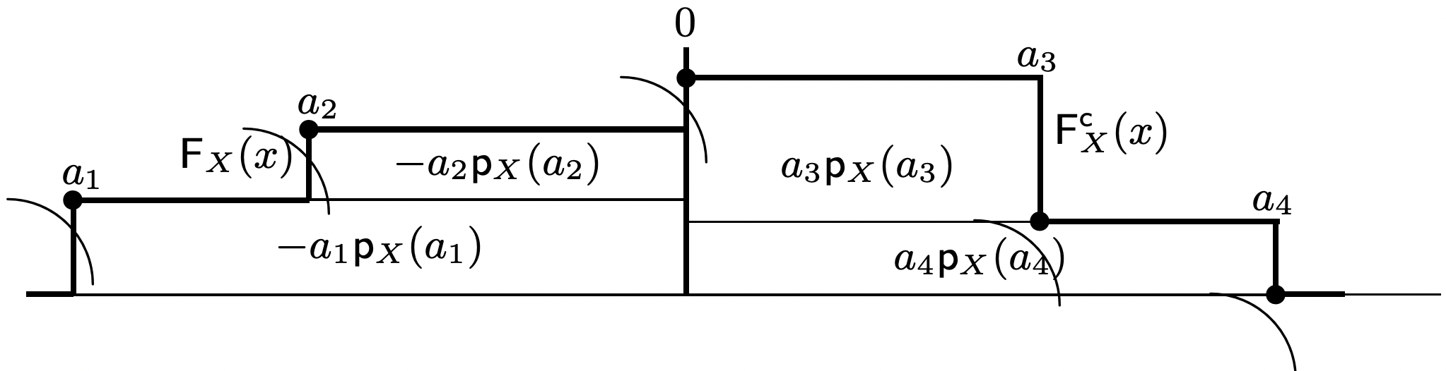
The first integral in \ref{1.35} corresponds to the negative sample values and the second to the positive sample values, and E [X] exists if and only if both integrals are finite (i.e., if E [|X|] is finite.

For continuous valued rv’s with positive and negative sample values, the conventional definition of expectation (assuming that E [|X|] exists) is given by

\[\mathrm{E}[X]=\int_{-\infty}^{\}\infty} x \mathrm{f}_{X}(x) d x\label{1.36} \]

This is equal to \ref{1.35} by the same argument as with nonnegative rv’s. Also, as with nonnegative rv’s, \ref{1.35} also applies to arbitrary rv’s. We thus have the following fundamental definition of expectation:

Definition 1.3.7. The expectation E [X] of a rv \(X\) exists, with the value given in (1.35), if each of the two terms in \ref{1.35} is finite. The expectation does not exist, but has value \(\infty\) \((-\infty)\), if the first term is finite (infinite) and the second infinite (finite). The expectation does not exist and is undefined if both terms are infinite.

We should not view the general expression in \ref{1.35} for expectation as replacing the need for the conventional expressions in \ref{1.36} and \ref{1.34} for continuous and discrete rv’s respectively. We will use all of these expressions frequently, using whichever is most convenient. The main advantages of \ref{1.35} are that it applies equally to all rv’s and that it poses no questions about convergence.

Example 1.3.3. The Cauchy rv \(X\) is the classic example of a rv whose expectation does not exist and is undefined. The probability density is \(\mathrm{f}_{X}(x)=\frac{1}{\pi\left(1+x^{2}\right)}\). Thus \(x \mathrm{f}_{X}(x)\) is proportional to \(1 / x\) both as \(x \rightarrow \infty\) and as \(x \rightarrow-\infty\). It follows that \(\int_{0}^{\infty} x f_{X}(x) d x\) and \(\int_{-\infty}^{0}-x f_{X}(x) d x\) are both infinite. On the other hand, we see from symmetry that the Cauchy principal value of the integral in \ref{1.36} is given by

\(\lim _{A \rightarrow \infty} \int_{-A}^{\}A} \frac{x}{\pi(1+x)^{2}} d x=0\)

There is usually little motivation for considering the upper and lower limits of the integration to have the same magnitude, and the Cauchy principal value usually has little significance for expectations.

Random variables as functions of other random variables

Random variables (rv’s) are often defined in terms of each other. For example, if \(h\) is a function from \(\mathbb{R}\) to \(\mathbb{R}\) and \(X\) is a rv, then \(Y=h(X)\) is the random variable that maps each sample point \(\omega\) to the composite function \(h(X(\omega))\). The distribution function of \(Y\) can be found from this, and the expected value of \(Y\) can then be evaluated by (1.35).

It is often more convenient to find E [Y] directly using the distribution function of \(X\). Exercise 1.16 indicates that E [Y] is given by \(\left.\int\right\} h(x) \mathrm{f}_{X}(x) d x\) for continuous rv’s and by \(\sum_{x} h(x) \mathrm{p}_{X}(x)\) for discrete rv’s. In order to avoid continuing to use separate expressions for continuous and discrete rv’s, we express both of these relations by

\[\mathrm{E}[Y]=\int_{-\infty}^{\}\infty} h(x) d \mathrm{~F}_{X}(x)\label{1.37} \]

This is known as a Stieltjes integral, which can be used as a generalization of both the continuous and discrete cases. For most purposes, we use Stieltjes integrals²² as a notational shorthand for either \(\left.\int\right\} h(x) \mathrm{f}_{X}(x) d x\) or \(\sum_{x} h(x) \mathrm{p}_{X}(x)\).

Knowing that E [X] exists does not guarantee that E [Y] exists, but we will treat the question of existence as it arises rather than attempting to establish any general rules.

Particularly important examples of such expected values are the moments \(\mathrm{E}\left[X^{n}\right]\) of a rv X and the central moments \(\left.\mathrm{E}\left[(X-\bar{X})^{n}\right]\right\}\) of \(X\), where \(\bar{X}\) is the mean \(\mathrm{E}[X]\). The second central moment is called the variance, denoted by \(\sigma_{X}^{2}\) or VAR[X]. It is given by

\[\left.\sigma_{X}^{2}=\mathrm{E}\left[(X-\bar{X})^{2}\right]\right\} \mathrm{E}\left[X^{2}\right]-\bar{X}^{2}\label{1.38} \]

The standard deviation \(\sigma_{X}\) of \(X\) is the square root of the variance and provides a measure of dispersion of the rv around the mean. Thus the mean is a rough measure of typical values for the outcome of the rv, and \(\sigma_{X}\) is a measure of the typical difference between \(X\) and \(\bar{X}\). There are other measures of typical value (such as the median and the mode) and other measures of dispersion, but mean and standard deviation have a number of special properties that make them important. One of these (see Exercise 1.21) is that \(\left.\mathrm{E}\left[(X-a)^{2}\right]\right\}\) is minimized over \(\alpha\) when \(\alpha=\mathrm{E}[X]\).

Next suppose \(X\) and \(Y\) are rv’s and consider the \(\mathrm{rv}^{23} Z=X+Y\). If we assume that \(X\) and \(Y\) are independent, then the distribution function of \(Z=X+Y\) is given by²⁴

\[\mathrm{F}_{Z}(z)=\int_{-\infty}^{\}\infty} \mathrm{F}_{X}(z-y) d \mathrm{~F}_{Y}(y)=\int_{-\infty}^{\}\infty} \mathrm{F}_{Y}(z-x) d \mathrm{~F}_{X}(x)\label{1.39} \]

If \(X\) and \(Y\) both have densities, this can be rewritten as

\[\mathrm{f}_{Z}(z)=\int_{-\infty}^{\}\infty} \mathrm{f}_{X}(z-y) \mathrm{f}_{Y}(y) d y=\int_{-\infty}^{\}\infty} \mathrm{f}_{Y}(z-x) \mathrm{f}_{X}(x) d x\label{1.40} \]

Eq. \ref{1.40} is the familiar convolution equation from linear systems, and we similarly refer to \ref{1.39} as the convolution of distribution functions (although it has a different functional form from (1.40)). If \(X\) and \(Y\) are nonnegative random variables, then the integrands in \ref{1.39} and \ref{1.40} are non-zero only between 0 and \(z\), so we often use 0 and \(z\) as the limits in \ref{1.39} and (1.40).

If \(X_{1}, X_{2}, \ldots, X_{n}\) are independent rv’s, then the distribution of the rv \(S_{n}=X_{1}+X_{2}+\cdots+X_n\) can be found by first convolving the distributions of \(X_{1}\) and \(X_{2}\) to get the distribution of \(S_{2}\) and then, for each \(i \geq 2\), convolving the distribution of \(S_{i}\) and \(X_{i+1}\) to get the distribution of \(S_{i+1}\). The distributions can be convolved in any order to get the same resulting distribution.

Whether or not \(X_{1}, X_{2}, \ldots, X_{n}\) are independent, the expected value of \(S_{n}=X_{1}+X_{2}+\dots+X_n\) satisfies

\[\mathrm{E}\left[S_{n}\right]=\mathrm{E}\left[X_{1}+X_{2}+\cdots+X_{n}\right]=\mathrm{E}\left[X_{1}\right]+\mathrm{E}\left[X_{2}\right]+\cdots+\mathrm{E}\left[X_{n}\right]\label{1.41} \]

This says that the expected value of a sum is equal to the sum of the expected values, whether or not the rv’s are independent (see exercise 1.11). The following example shows how this can be a valuable problem solving aid with an appropriate choice of rv’s.

Example 1.3.4. Consider a switch with n input nodes and n output nodes. Suppose each input is randomly connected to a single output in such a way that each output is also connected to a single input. That is, each output is connected to input 1 with probability 1/n. Given this connection, each of the remaining outputs are connected to input 2 with probability 1/(n 1), and so forth.

An input node is said to be matched if it is connected to the output of the same number. We want to show that the expected number of matches (for any given n) is 1. Note that the first node is matched with probability 1/n, and therefore the expectation of a match for node 1 is 1/n. Whether or not the second input node is matched depends on the choice of output for the first input node, but it can be seen from symmetry that the marginal distribution for the output node connected to input 2 is 1/n for each output. Thus the expectation of a match for node 2 is also 1/n. In the same way, the expectation of a match for each input node is 1/n. From (1.41), the expected total number of matchs is the sum over the expected number for each input, and is thus equal to 1. This exercise would be quite difficult without the use of (1.41).

If the rv’s \(X_{1}, \ldots, X_{n}\) are independent, then, as shown in exercises 1.11 and 1.18, the variance of \(S_{n}=X_{1}+\cdots+X_{n}\) is given by

\[\sigma_{S_{n}}^{2}=\sum_{i=1}^{n} \sigma_{X_{i}}^{2}\label{1.42} \]

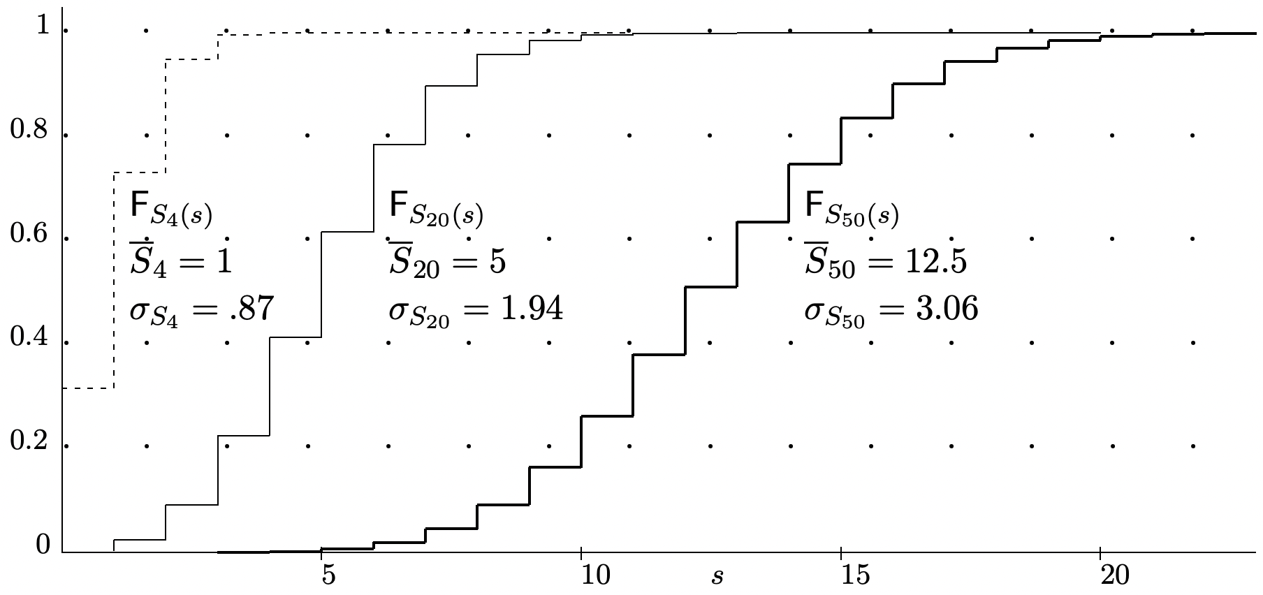
If \(X_{1}, \ldots, X_{n}\) are also identically distributed (i.e., \(X_{1}, \ldots, X_{n}\) are IID) with variance \(\sigma_{X}^{2}\), then \(\sigma_{S_{n}}^{2}=n \sigma_{X}^{2}\). Thus the standard deviation of \(S_{n}\) is \(\sigma_{S_{n}}=\sqrt{n} \sigma_{X}\). Sums of IID rv’s 2 appear everywhere in probability theory and play an especially central role in the laws of large numbers. It is important to remember that the mean of \(S_{n}\) is linear in \(n\) but the standard deviation increases only with the square root of \(n\). Figure 1.5 illustrates this behavior.

Figure 1.5: The distribution function \(\mathrm{F}_{S_{n}}(s)\) of \(S_{n}=X_{1}+\cdots+X_{n}\) where \(X_{1}, \ldots, X_{n}\) are typical IID rv’s and \(n\) takes the values 4, 20, and 50. The particular rv in the figure is binary with pX(1) = 1/4, pX(0) = 3/4. Note that the mean of \(S_{n}\) is proportional to \(n\) and the standard deviation to \(\sqrt{n}\).

Conditional expectations

Just as the conditional distribution of one rv conditioned on a sample value of another rv is important, the conditional expectation of one rv based on the sample value of another is equally important. Initially let X be a positive discrete rv and let y be a sample value of another discrete rv Y such that pY \ref{y} > 0. Then the conditional expectation of X given Y = y is defined to be

\[\mathrm{E}[X \mid Y=y]=\sum_{x} x \mathrm{p}_{X \mid Y}(x \mid y)\label{1.43} \]

This is simply the ordinary expected value of X using the conditional probabilities in the reduced sample space corresponding to Y = y. This value can be finite or infinite as before. More generally, if X can take on positive or negative values, then there is the possibility that the conditional expectation is undefined. In other words, for discrete rv’s, the conditional expectation is exactly the same as the ordinary expectation, except that it is taken using conditional probabilities over the reduced sample space.

More generally yet, let X be an arbitrary rv and let y be a sample value of a discrete rv Y with \(\mathrm{p}_{Y}(y)>0\). The conditional distribution function of X conditional on Y = y is defined as

\(\mathrm{F}_{X \mid Y}(x \mid y)=\frac{\operatorname{Pr}\{X \leq x, Y=y\}}{\operatorname{Pr}\{Y=y\}}\)

Since this is an ordinary distribution function in the reduced sample space where Y = y, \ref{1.35} expresses the expectation of X conditional on Y = y as

\[\mathrm{E}[X \mid Y=y]=-\int_{-\infty}^{\}0} \mathrm{~F}_{X \mid Y}(x \mid y) d x+\int_{0}^{\}\infty} \mathrm{F}_{X \mid Y}(x \mid y) d x\label{1.44} \]

The forms of conditional expectation in \ref{1.43} and \ref{1.44} are given for individual sample values of Y for which \(\mathrm{p}_{Y}(y)>0\).

We next show that the conditional expectation of X conditional on a discrete rv Y can also be viewed as a rv. With the possible exception of a set of zero probability, each \(\omega \in \Omega\) maps to {Y = y} for some y with \(\mathrm{p}_{Y}(y)>0\) and \(\mathrm{E}[X \mid Y=y]\) is defined for that y. Thus we can define \(\mathrm{E}[X \mid Y] \mathrm{as}^{25}\) a rv that is a function of Y , mapping \(\omega\) to a sample value, say y of Y, and mapping that y to \(\mathrm{E}[X \mid Y=y]\). Regarding a conditional expectation as a rv that is a function of the conditioning rv is a powerful tool both in problem solving and in advanced work. For now, we use this to express the unconditional mean of X as

\[\mathrm{E}[X]=\mathrm{E}[\mathrm{E}[X \mid Y]]\label{1.45} \]

where the inner expectation is over X for each value of Y and the outer expectation is over the rv E [X | Y ], which is a function of Y.

Example 1.3.5. Consider rolling two dice, say a red die and a black die. Let \(X_{1}\) be the number on the top face of the red die, and \(X_{2}\) that for the black die. Let \(S=X_{1}+X_{2}\). Thus \(X_{1}\) and \(X_{2}\) are IID integer rv’s, each uniformly distributed from 1 to 6. Conditional on \(S=j\), \(X_{1}\) is uniformly distributed between 1 and \(j-1\) for \(j \leq 7\) and between \(j-6\) and 6 for \(j \geq 7\). For each \(j \leq 7\), it follows that \(\mathrm{E}\left[X_{1} \mid S=j\right]=j / 2\). Similarly, for \(j \geq 7\), \(\mathrm{E}\left[X_{1} \mid S=j\right]=j / 2\). This can also be seen by the symmetry between \(X_{1}\) and \(X_{2}\).

The rv \(\mathrm{E}\left[X_{1} \mid S\right]\) is thus a discrete rv taking on values from 1 to 6 in steps of 1/2 as the sample value of | S goes from 2 to 12. The PMF of \(\mathrm{E}\left[X_{1} \mid S\right]\) is given by \(\mathrm{p}_{\mathrm{E}\left[X_{1} \mid S\right]}(j / 2)=\mathrm{p}_{S}(j)\). Using (1.45), we can then calculate \(\mathrm{E}\left[X_{1}\right]\) as

\(\left.\left.\mathrm{E}\left[X_{1}\right]=\mathrm{E}\left[\mathrm{E}\left[X_{1} \mid S\right]\right]\right\}=\sum_{j=2}^{12}\right\} \frac{j}{2} \mathrm{p}_{S}(j)=\frac{\mathrm{E}[S]}{2}=\frac{7}{2}\)

This example is not intended to show the value of \ref{1.45} in calculating expectation, since \(\mathrm{E}\left[X_{1}\right]=7 / 2\) is initially obvious from the uniform integer distribution of \(X_{1}\). The purpose is simply to illustrate what the rv \(\mathrm{E}\left[X_{1} \mid S\right]\) means.

To illustrate \ref{1.45} in a more general way, while still assuming X to be discrete, we can write out this expectation by using \ref{1.43} for \(\mathrm{E}[X \mid Y=y]\).

\[\begin{aligned}
\mathrm{E}[X] &=\mathrm{E}[\mathrm{E}[X \mid Y]]\}=\sum_{y} \mathrm{p}_{Y}(y) \mathrm{E}[X \mid Y=y] \\
&=\sum_{y} \mathrm{p}_{Y}(y) \sum_{x} x \mathrm{p}_{X \mid Y}(x \mid y)
\end{aligned}\label{1.46} \]

Operationally, there is nothing very fancy in the example or in (1.45). Combining the sums, \ref{1.46} simply says that \(\mathrm{E}[X]=\sum_{y, x} x \mathrm{p}_{Y X}(y, x)\). As a concept, however, viewing the conditional expectation \(\mathrm{E}[X \mid Y]\) as a rv based on the conditioning rv Y is often a useful theoretical tool. This approach is equally useful as a tool in problem solving, since there are many problems where it is easy to find conditional expectations, and then to find the total expectation by averaging over the conditioning variable. For this reason, this result is sometimes called either the total expectation theorem or the iterated expectation theorem. Exercise 1.17 illustrates the advantages of this approach, particularly where it is initially unclear whether or not the expectation is finite. The following cautionary example, however, shows that this approach can sometimes hide convergence questions and give the wrong answer.

Example 1.3.6. Let Y be a geometric rv with the \(\mathrm{PMF} \mathrm{p}_{Y}(y)=2^{-y}\) for integer \(y \geq 1\). Let X be an integer rv that, conditional on Y , is binary with equiprobable values \(\pm 2^{y}\) given Y = y. We then see that \(\mathrm{E}[X \mid Y=y]=0\) for all y, and thus, \ref{1.46} indicates that \(\mathrm{E}[X]=0\). On the other hand, it is easy to see that \(\mathrm{p}_{X}\left(2^{k}\right)=\mathrm{p}_{X}\left(-2^{k}\right)=2^{-k-1}\) for each integer \(k \geq 1\). Thus the expectation over positive values of X is \(\infty\) and that over negative values is \(-\infty\). In other words, the expected value of X is undefined and \ref{1.46} is incorrect.

The diculty in the above example cannot occur if X is a nonnegative rv. Then \ref{1.46} is simply a sum of a countable number of nonnegative terms, and thus it either converges to a finite sum independent of the order of summation, or it diverges to \(\infty\), again independent of the order of summation.

If X has both positive and negative components, we can separate it into \(X=X^{+}+X^{-}\) where \(X^{+}=\max (0, X)\) and \(X^{-}=\min (X, 0)\). Then \ref{1.46} applies to \(X^{+}\) and \(-X^{-}\) separately. If at most one is infinite, then \ref{1.46} applies to X, and otherwise X is undefined. This is summarized in the following theorem:

Theorem 1.3.1 (Total expectation). Let X and Y be discrete rv’s. If X is nonnegative, then \(\mathrm{E}[X]=\mathrm{E}[\mathrm{E}[X \mid Y]]\}=\sum_{y} \mathrm{p}_{Y}(y) \mathrm{E}[X \mid Y=y]\). If X has both positive and negative values, and if at most one of \(\mathrm{E}\left[X^{+}\right]\) and \(\mathrm{E}\left[-X^{-}\right]\) is infinite, then \(\mathrm{E}[X]=\mathrm{E}[\mathrm{E}[X \mid Y]]\}=\sum_y\mathrm{p_Y}(y)\mathrm{E[X|Y]=}y]\).

We have seen above that if Y is a discrete rv, then the conditional expectation \(\mathrm{E}[X \mid Y=y]\) is little more complicated than the unconditional expectation, and this is true whether X is discrete, continuous, or arbitrary. If X and Y are continuous, we can essentially extend these results to probability densities. In particular, defining \(\mathrm{E}[X \mid Y=y]\) as

\[\mathrm{E}[X \mid Y=y]=\int_{-\infty}^{\}\infty} x \mathrm{f}_{X \mid Y}(x \mid y)\label{1.47} \]

we have

\[\mathrm{E}[X]=\int_{-\infty}^{\}\infty} \mathrm{f}_{Y}(y) \mathrm{E}[X \mid Y=y] d y=\int_{-\infty}^{\}\infty} \mathrm{f}_{Y}(y) \int_{-\infty}^{\}\infty} x \mathrm{f}_{X \mid Y}(x \mid y) d x d y\label{1.48} \]

We do not state this as a theorem because the details about the integration do not seem necessary for the places where it is useful.

Indicator random variables

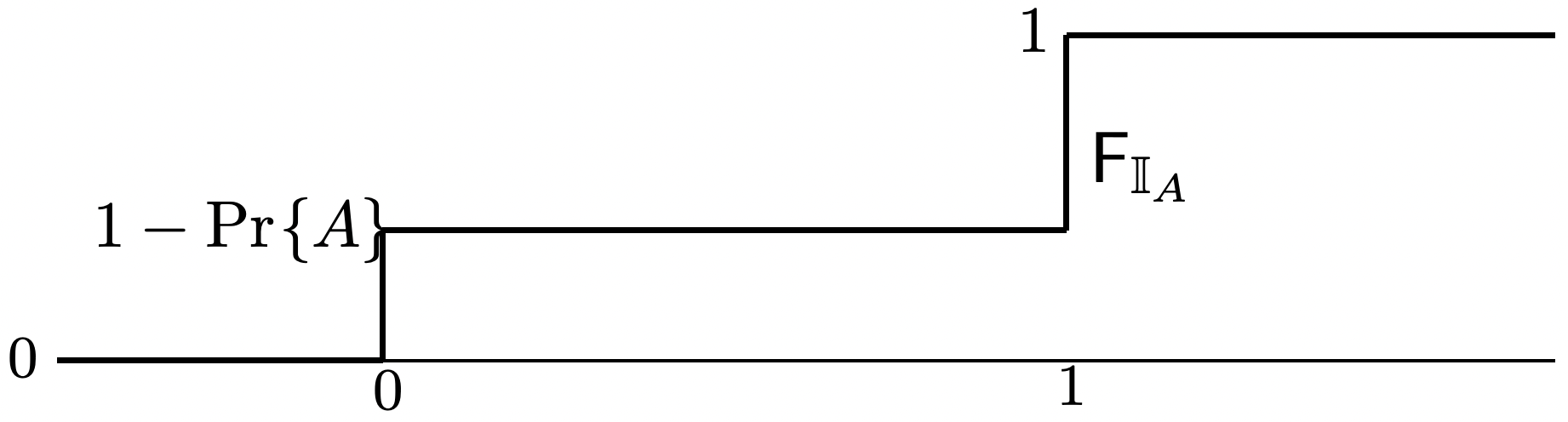
For any event A, the indicator random variable of A, denoted \(\mathbb{I}_{A}\), is a binary rv that has the value 1 for all \(\omega \in A\) and the value 0 otherwise. It then has the \(\operatorname{PMF} \mathrm{p}_{\mathbb{I}_{A}}(1)=\operatorname{Pr}\{A\}\) and \(\mathrm{p}_{\mathbb{I}_{A}}(0)=1-\operatorname{Pr}\{A\}\). The corresponding distribution function \(\mathrm{F}_{\mathbb{I}_{A}}\) is then illustrated in Figure 1.6. It is easily seen that \(\mathrm{E}\left[\mathbb{I}_{A}\right]=\operatorname{Pr}\{A\}\).

Figure 1.6: The distribution function \(\mathrm{F}_{\mathbb{I}_{A}}\) of an indicator random variable \(\mathbb{I}_{A}\).

Indicator rv’s are useful because they allow us to apply the many known results about rv’s and particularly binary rv’s to events. For example, the laws of large numbers are expressed in terms of sums of rv’s, and those results all translate into results about relative frequencies through the use of indicator functions.

Moment generating functions and other transforms

The moment generating function (MGF) for a rv X is given by

\[\left.\mathrm{g}_{X}(r)=\mathrm{E}\left[e^{r X}\right]\right\} =\int_{-\infty}^{\}\infty} e^{r x} d \mathrm{~F}_{X}(x)\label{1.49} \]

where r is a real variable. The integrand is nonnegative, and we can study where the integral exists (i.e., where it is finite) by separating it as follows:

\[\mathrm{g}_{X}(r)=\int_{0}^{\}\infty} e^{r x} d \mathrm{~F}_{X}(x)+\int_{-\infty}^{\}0} e^{r x} d \mathrm{~F}_{X}(x)\label{1.50} \]

Both integrals exist for \(r=0\), since the first is \(\operatorname{Pr}\{X>0\}\) and the second is \(\operatorname{Pr}\{X \leq 0\}\). The first integral is increasing in r, and thus if it exists for one value of r, it also exists for all smaller values. For example, if X is a nonnegative exponential rv with the density \(\mathrm{f}_{X}(x)=e^{-x}\), then the first integral exists if and only \(r<1\), where it has the value \(\frac{1}{1-r}\). As another example, if X satisfies Pr{X > A} = 0 for some finite A, then the first integral is at most \(e^{r A}\), which is finite for all real r.

Let \(r_{+}(X)\) be the supremum of values of \(r\) for which the first integral exists. The first integral exists for all \(r<r_{+}(X)\), and \(0 \leq r_{+}(X) \leq \infty\). In the same way, let \(r_{-}(X)\) be the infimum of values of \(r\) for which the the second integral exists. The second integral exists for all \(r>r_{-}(X)\) and \(r_{-}(X)\) satisfies \(0 \geq r_{-}(X) \geq-\infty\).

Combining the two integrals, the region over which the MGF of an arbitrary rv exists is an interval \(I(X)\) from \(r_{-}(X) \leq 0 \text { to } r_{+}(X) \geq 0\). Either or both of the end points, \(r_{-}(X)\) and \(r_{+}(X)\), might be included in \(I(X)\), and either or both might be either 0 or infinite. We denote these quantities as I, \(r_{-}\), and \(r_{+}\) when the rv X is clear from the context. Appendix A gives the interval I for for a number of standard rv’s and Exercise 1.22 illustrates I(X) further.

If gX(r) exists in an open region of r around 0 (i.e., if \(r_{-}<0<r_{+}\)), then derivatives²⁶ of all orders exist in that region. They are given by

\[\frac{\partial^{k} \mathrm{~g}_{X}(r)}{\partial r^{k}}=\int_{-\infty}^{\}\infty} x^{k} e^{r x} d \mathrm{~F}_{X}(x) \quad ;\left.\quad \frac{\partial^{k} \mathrm{~g}_{X}(r)}{\partial r^{k}}\right|_{r=0}=\mathrm{E}\left[X^{k}\right]\label{1.51} \]

This shows that finding the moment generating function often provides a convenient way to calculate the moments of a random variable. If any moment fails to exist, however, then the MGF must also fail to exist over each open interval containing 0 (see Exercise 1.31).

Another convenient feature of moment generating functions is their use in treating sums of independent rv’s. For example, let \(S_{n}=X_{1}+X_{2}+\cdots+X_{n}\). Then

\[\left.\left.\left.\mathrm{g}_{S_{n}}(r)=\mathrm{E}\left[e^{r S_{n}}\right]\right\} =\mathrm{E}\left[\exp \left(\sum_{i=1}^{n} r X_{i}\right)\right]\right\}=\mathrm{E}\left[\prod_{i=1}^{n} \exp \left(r X_{i}\right)\right]\right\} \prod_{i=1}^{n} \mathrm{~g}_{X_{i}}(r)\label{1.52} \]

In the last step here, we have used a result of Exercise 1.11, which shows that for independent rv’s, the mean of the product is equal to the product of the means. If \(X_{1}, \ldots, X_{n}\) are also IID, then

\[g_{S_{n}}(r)=\left[\mathrm{g}_{X}(r)\right]^{n}\label{1.53} \]

We will use this property frequently in treating sums of IID rv’s. Note that this also implies that the region over which the MGF’s of \(S_{n}\) and X exist are the same, i.e., \(I\left(S_{n}\right)=I(X)\).

The real variable r in the MGF can also be viewed as a complex variable, giving rise to a number of other transforms. A particularly important case is to view r as a pure imaginary variable, say \(i \omega\) where \(i=\sqrt{-1}\) and \(\omega\) is real. The MGF is then called the characteristic function. Since \(\left|e^{i \omega x}\right|\) is 1 for all \(x\), \(g_{X}(i \omega)\) exists for all rv’s X and all real \(\omega\), and its magnitude is at most one. Note that \(g_{X}(-i \omega)\) is the Fourier transform of the density of X, so the Fourier transform and characteristic function are the same except for this small notational difference.

The Z-transform is the result of replacing \(e^{r}\) with \(z\) in \(g_{X}(r)\). This is useful primarily for integer valued rv’s, but if one transform can be evaluated, the other can be found immediately. Finally, if we use \(-s\), viewed as a complex variable, in place of \(r\), we get the two sided Laplace transform of the density of the random variable. Note that for all of these transforms, multiplication in the transform domain corresponds to convolution of the distribution functions or densities, and summation of independent rv’s. The simplicity of taking products of transforms is a major reason that transforms are so useful in probability theory.

---

Reference

¹²For example, suppose \(\Omega\) is the closed interval [0, 1] of real numbers with a uniform probability distribution over [0, 1]. If \(X(\omega)=1 / \omega\), then the sample point 0 maps to \(\infty\) but \(X\) is still regarded as a rv. These subsets of 0 probability are usually ignored, both by engineers and mathematicians. Thus, for example, the set \(\{\omega \in \Omega: X(\omega) \leq x\}\) means the set for which \(X(\omega)\) is both defined and satisfies \(X(\omega) \leq x\).

¹³These last two modifications are technical limitations connected with measure theory. They can usually be ignored, since they are satisfied in all but the most bizarre conditions. However, just as it is important to know that not all subsets in a probability space are events, one should know that not all functions from \(\Omega\) to \(\mathbb{R}\) are rv’s.

¹⁴The distribution function is sometimes referred to as the cumulative distribution function.

¹⁵Stochastic and random are synonyms, but random has become more popular for rv’s and stochastic for stochastic processes. The reason for the author’s choice is that the common-sense intuition associated with randomness appears more important than mathematical precision in reasoning about rv’s, whereas for stochastic processes, common-sense intuition causes confusion much more frequently than with rv’s. The less familiar word stochastic warns the reader to be more careful.

¹⁶This definition is deliberately vague, and the choice of whether to call a sequence of rv’s a process or a sequence is a matter of custom and choice.

¹⁷We say that a sequence \(Y_{1}, Y_{2}, \ldots\), of rv’s are IID if for each integer \(n\), the rv’s \(Y_{1}, \ldots, Y_{n}\) are IID. There are some subtleties in going to the limit \(n \rightarrow \infty\), but we can avoid most such subtleties by working with finite \(n\)-tuples and going to the limit at the end.

¹⁸This is one of those maddening arguments that, while intuitively obvious, requires some careful reasoning to be completely convincing. We go through several similar arguments with great care in Chapter 2, and suggest that skeptical readers wait until then to prove this rigorously.

¹⁹Proofs with an asterisk can be omitted without an essential loss of continuity

²⁰See Feller [7] for a derivation of these results about the Stirling bounds. Feller also shows that that an improved lower bound to \(n !\) is given by \(\sqrt{2 \pi n}(n / e)^{n} \exp \left[\frac{1}{12 n}-\frac{1}{360 n^{3}}\right]\).

²²More specifically, the Riemann-Stieltjes integral, abbreviated here as the Stieltjes integral, is denoted as \(\int_{a}^{b} h(x) d F_{X}(x)\). This integral is defined as the limit of a generalized Riemann sum, \(\lim _{\delta \rightarrow 0} \sum_{n} h\left(x_{n}\right)\left[\mathrm{F}\left(y_{n}\right)-\right.\mathrm{F}(y_{n-1})]\) where \(\left\{y_{n} ; n \geq 1\right\}\) is a sequence of increasing numbers from a to b satisfying \(y_{n}-y_{n-1} \leq \delta\) and \(y_{n-1}<x_{n} \leq y_{n}\) for all \(n\) The Stieltjes integral exists over finite limits if the limit exists and is independent of the choices of \(\left\{y_{n}\right\}\) and \(\left\{x_{n}\right\}\) as \(\delta \rightarrow 0\). It exists over infinite limits if it exists over finite lengths and a limit over the integration limits can be taken. See Rudin [18] for an excellent elementary treatment of Stieltjes integration, and see Exercise 1.12 for some examples.

²³The question whether a real-valued function of rv’s is itself a rv is usually addressed by the use of measure theory, and since we neither use nor develop measure theary in this text, we usually simply assume (within the limits of common sense) that any such function is itself a rv. However, the sum \(X+Y\) of rv’s is so important throughout this subject that Exercise 1.10 provides a guided derivation of this result for \(X+Y\). In the same way, the sum \(S_{n}=X_{1}+\cdots+X_{n}\) of any finite collection of rv’s is also a rv.

²⁴See Exercise 1.12 for some peculiarties about this definition.

²⁵This assumes that \(\mathrm{E}[X \mid Y=y]\) is finite for each y, which is one of the reasons that expectations are said to exist only if they are finite.

²⁶This result depends on interchanging the order of differentiation (with respect to \(r\)) and integration (with respect to \(x\)). This can be shown to be permissible because \(\mathrm{g}_{X}(r)\) exists for \(r\) both greater and smaller than 0, which in turn implies, first, that \(1-\mathrm{F}_{X}(x)\) must approach 0 exponentially as \(x \rightarrow \infty\) and, second, that \(\mathrm{F}_{X}(x)\) must approach 0 exponentially as \(x \rightarrow-\infty\).