1.4: Basic Inequalities

Inequalities play a particularly fundamental role in probability, partly because many of the models we study are too complex to find exact answers, and partly because many of the most useful theorems establish limiting rather than exact results. In this section, we study three related inequalities, the Markov, Chebyshev, and Chernoff bounds. These are used repeatedly both in the next section and in the remainder of the text.

Markov Inequality

This is the simplest and most basic of these inequalities. It states that if a nonnegative random variable \(Y\) has a mean \(\mathrm{E}[Y]\), then, for every \(y>0\), \(\operatorname{Pr}\{Y \geq y\}\) satisfies²⁷

\[\operatorname{Pr}\{Y \geq y\} \leq \frac{\mathrm{E}[Y]}{y} \quad \text { Markov Inequality for nonnegative } Y\label{1.54} \]

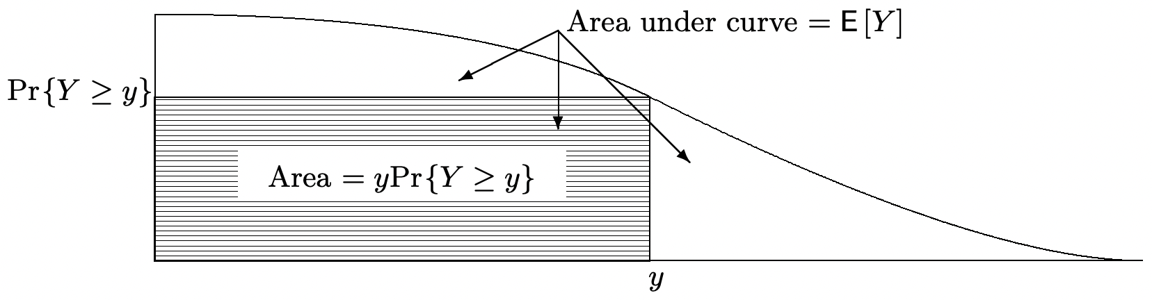
Figure 1.7 derives this result using the fact (see Figure 1.3) that the mean of a nonnegative rv is the integral of its complementary distribution function, i.e., of the area under the curve \(\operatorname{Pr}\{Y>z\}\). Exercise 1.28 gives another simple proof using an indicator random variable.

As an example of this inequality, assume that the average height of a population of people is 1.6 meters. Then the Markov inequality states that at most half of the population have a height exceeding 3.2 meters. We see from this example that the Markov inequality is often very weak. However, for any \(y>0\), we can consider a rv that takes on the value \(y\) with probability \(\epsilon\) and the value 0 with probability \(1-\epsilon\); this rv satisfies the Markov inequality at the point \(y\) with equality. Figure 1.7 (as elaborated in Exercise 1.40) also shows that, for any nonnegative rv Y with a finite mean,

\[\lim _{y \rightarrow \infty} y \operatorname{Pr}\{Y \geq y\}=0\label{1.55} \]

This will be useful shortly in the proof of Theorem 1.5.3.

Figure 1.7: Demonstration that \(y \operatorname{Pr}\{Y \geq y\} \leq \mathrm{E}[Y]\). By letting \(y \rightarrow \infty\), it can also be seen that the shaded area becomes a negligible portion of the area \(\mathrm{E}[Y]\), so that \(\lim _{y \rightarrow \infty} y \operatorname{Pr}\{Y>y\}=0 \text { if } \mathrm{E}[Y]<\infty\)

Chebyshev inequality

We now use the Markov inequality to establish the well-known Chebyshev inequality. Let \(Z\) be an arbitrary rv with finite mean \(\mathrm{E}[Z]\) and finite variance \(\sigma_{Z}^{2}\), and define \(Y\) as the nonnegative rv \(Y=(Z-\mathrm{E}[Z])^{2}\). Thus \(\mathrm{E}[Y]=\sigma_{Z}^{2}\). Applying (1.54),

\(\operatorname{Pr}\left\{(Z-\mathrm{E}[Z])^{2} \geq y \leq \frac{\sigma_{Z}^{2}}{y} \quad \text { for any } y>0\right.\)

Replacing y with \(\epsilon^{2}\) (for any \(\epsilon>0\)) and noting that the event \(\left\{(Z-\mathrm{E}[Z])^{2} \geq \epsilon^{2}\right\}\) is the same as \(|Z-\mathrm{E}[Z]| \geq \epsilon\), this becomes

\[\operatorname{Pr}\{|Z-\mathrm{E}[Z]| \geq \epsilon\} \leq \frac{\sigma_{Z}^{2}}{\epsilon^{2}} \quad(\text { Chebyshev inequality })\label{1.56} \]

Note that the Markov inequality bounds just the upper tail of the distribution function and applies only to nonnegative rv’s, whereas the Chebyshev inequality bounds both tails of the distribution function. The more important difference, however, is that the Chebyshev bound goes to zero inversely with the square of the distance from the mean, whereas the Markov bound goes to zero inversely with the distance from 0 (and thus asymptotically with distance from the mean).

The Chebyshev inequality is particularly useful when \(Z\) is the sample average, \(\left(X_{1}+X_{2}+\dots X_n\right.)/n\), of a set of IID rv’s. This will be used shortly in proving the weak law of large numbers.

Chernoff bounds

Chernoff (or exponential) bounds are another variation of the Markov inequality in which the bound on each tail of the distribution function goes to 0 exponentially with distance from the mean. For any given rv \(Z\), let \(I(Z)\) be the interval over which the \(\left.\operatorname{MGF} g_{Z}(r)=\mathrm{E}\left[e^{Z r}\right]\right\}\) exists. Letting \(Y=e^{Z r}\) for any \(r \in I(Z)\), the Markov inequality \ref{1.54} applied to \(Y\) is

\(\operatorname{Pr}\{\exp (r Z) \geq y\} \leq \frac{\mathrm{g}_{Z}(r)}{y} \quad \text { for any } y>0\)

This takes on a more meaningful form if \(y\) is replaced by \(e^{r b}\). Note that exp \((r Z) \geq \exp (r b)\) is equivalent to \(Z \geq b\) for \(r>0\) and to \(Z<b\) for \(r<0\). Thus, for any real \(b\), we get the following two bounds, one for \(r>0\) and the other for \(r<0\):

\[\operatorname{Pr}\{Z \geq b\} \leq g_{Z}(r) \exp (-r b) ; \quad \text { (Chernoff bound for } 0<r \in I(Z)\label{1.57} \]

\[\left.\operatorname{Pr}\{Z \leq b\} \leq g_{Z}(r) \exp (-r b) ; \quad \text { (Chernoff bound for } 0>r \in I(Z)\right)\label{1.58} \]

This provides us with a family of upper bounds on the tails of the distribution function, using values of \(r>0\) for the upper tail and \(r<0\) for the lower tail. For fixed \(0<r \in I(Z)\), this bound on \(\operatorname{Pr}\{Z \geq b\}\) decreases exponentially²⁸ in \(b\) at rate \(r\). Similarly, for each \(0>r \in I(Z)\), the bound on \(\operatorname{Pr}\{Z \leq b\}\) decreases exponentially at rate \(r\) as \(b \rightarrow-\infty\). We will see shortly that \ref{1.57} is useful only when \(b>\mathrm{E}[X]\) and \ref{1.58} is useful only when \(b<\mathrm{E}[X])\).

The most important application of these Chernoff bounds is to sums of IID rv’s. Let \(S_{n}=X_{1}+\cdots+X_{n}\) where \(X_{1}, \ldots, X_{n}\) are IID with the MGF \(\mathrm{g}_{X}(r)\). Then \(\mathrm{g}_{S_{n}}(r)=\left[\mathrm{g}_{X}(r)\right]^{n}\), so \ref{1.57} and \ref{1.58} (with \(b\) replaced by \(na\)) become

\[\operatorname{Pr}\left\{S_{n} \geq n a\right\} \leq\left[\mathrm{g}_{X}(r)\right]^{n} \exp (-r n a) ; \quad(\text { for } 0<r \in I(Z))\label{1.59} \]

\[\operatorname{Pr}\left\{S_{n} \leq n a\right\} \leq\left[\mathrm{g}_{X}(r)\right]^{n} \exp (-r n a) ; \quad(\text { for } 0>r \in I(Z))\label{1.60} \]

These equations are easier to understand if we define the semi-invariant MGF, \(\gamma_{X}(r)\), as

\[\gamma_{X}(r)=\ln g_{X}(r)\label{1.61} \]

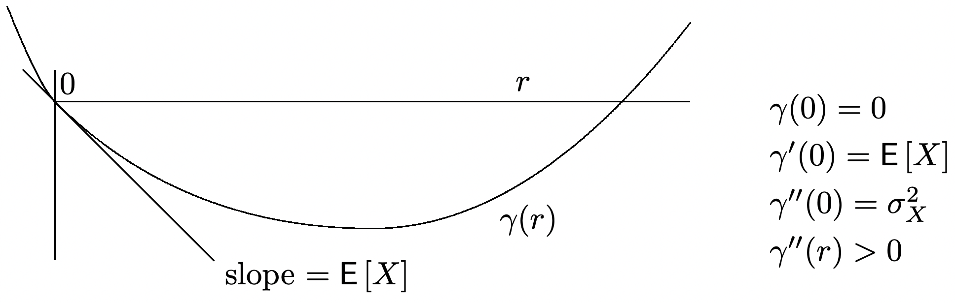
The semi-invariant MGF for a typical rv \(X\) is sketched in Figure 1.8. The major features to observe are, first, that \(\gamma_{X}^{\prime}(0)=\mathrm{E}[X]\) and, second, that \(\gamma_{X}^{\prime \prime}(r) \geq 0\) for \(r\) in the interior of \(I(X)\)..

Figure 1.8: Semi-invariant moment-generating function \(\gamma(r)\) for a typical rv \(X\) assum­ing \(r_{-}<0<r_{+}\). Since \(\gamma(r)=\ln g(r)\), we see that that \(\frac{\partial}{\partial r} \gamma(r)=\frac{1}{g(r)} \frac{\partial}{\partial r} g(r)\). Thus \(\gamma^{\prime}(0)=\mathrm{E}[X]\). Also, for \(r\) in the interior of \(I(X)\), Exercise 1.24 shows that \(\gamma^{\prime \prime}(r) \geq 0\), and in fact, \(\gamma^{\prime \prime}(r)\) is strictly positive except in the uninteresting case where \(X\) is deterministic (takes on a single value with probability 1). As indicated in the figure, the straight line of slope \(\mathrm{E}[X]\) through the origin is tangent to \(\gamma(r)\).

In terms of \(\gamma_{X}(r)\), \ref{1.59} and \ref{1.60} become

\[\operatorname{Pr}\left\{S_{n} \geq n a\right\} \leq \exp \left(n\left[\gamma_{X}(r)-r a\right]\right) ; \quad(\text { for } 0<r \in I(X)\label{1.62} \]

\[\operatorname{Pr}\left\{S_{n} \leq n a\right\} \leq \exp \left(n\left[\gamma_{X}(r)-r a\right]\right) ; \quad(\text { for } 0>r \in I(X)\label{1.63} \]

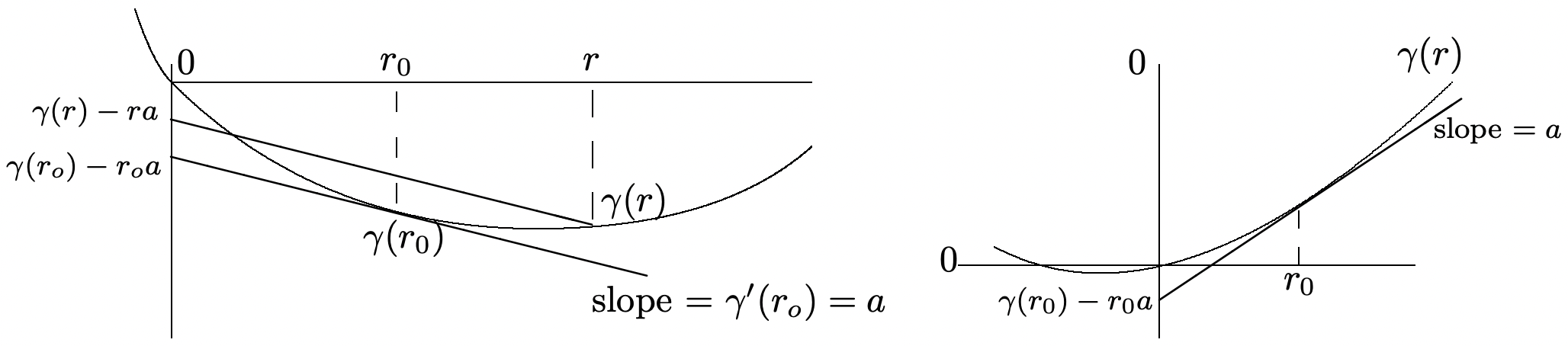
These bounds are geometric in \(n\) for fixed \(a\) and \(r\), so we should ask what value of \(r\) provides the tightest bound for any given \(a\). Since \(\gamma_{X}^{\prime \prime}(r)>0\), the tightest bound arises either at that \(r\) for which \(\gamma^{\prime}(r)=a\) or at one of the end points, \(r_{-}\) or \(r_{+}\), of \(I(X)\). This minimum value is denoted by

\(\mu_{X}(a)=\inf _{r}\left[\gamma_{X}(r)-r a\right]\)

Note that \(\left.\left(\gamma_{X}(r)-r a\right)\right|_{r=0}=0\) and \(\left.\frac{\partial}{\partial r}\left(\gamma_{X}(r)-r a\right)\right|_{r=0}=\mathrm{E}[X]-a\). Thus if \(a>E[X]\), then \(\gamma_{X}(r)-r a\) must be negative for suciently small positive \(r\). Similarly, if \(a<\mathrm{E}[X]\), then \(\gamma_{X}(r)-r a\) is negative for negative \(r\) suciently close²⁹ to 0. In other words,

\[\operatorname{Pr}\left\{S_{n} \geq n a\right\} \leq \exp \left(n \mu_{X}(a)\right) ; \quad \text { where } \mu_{X}(a)<0 \text { for } a>\mathrm{E}[X]\label{1.64} \]

\[\operatorname{Pr}\left\{S_{n} \leq n a\right\} \leq \exp \left(n \mu_{X}(a)\right) ; \quad \text { where } \mu_{X}(a)<0 \text { for } a<\mathrm{E}[X]\label{1.65} \]

This is summarized in the following lemma:

Lemma 1.4.1. Assume that 0 is in the interior of \(I(X)\) and let \(S_{n}\) be the sum of \(n\) IID rv’s each with the distribution of \(X\). Then \(\mu_{X}(a)=\inf _{r}\left[\gamma_{X}(r)-r a\right]<0\) for all \(a \neq \mathrm{E}[X]\). Also, \(\operatorname{Pr}\left\{S_{n} \geq n a\right\} \leq e^{n \mu_{X}(a)}\) for \(a>E[X]\) and \(\operatorname{Pr}\left\{S_{n} \leq n a\right\} \leq e^{n \mu_{X}(a)}\) for \(a<\mathrm{E}[X]\).

Figure 1.9 illustrates the lemma and gives a graphical construction to find³⁰ \(\mu_{X}(a)=\mathrm{inf}_r[\gamma_X(r)-ra]\).

These Chernoff bounds will be used in the next section to help understand several laws of large numbers. They will also be used extensively in Chapter 7 and are useful for detection, random walks, and information theory.

The following example evaluates these bounds for the case where the IID rv’s are binary. We will see that in this case the bounds are exponentially tight in a sense to be described.

Example 1.4.1. Let \(X\) be binary with \(\mathrm{p}_{X}(1)=p\) and \(\mathrm{p}_{X}(0)=q=1-p\). Then \(g_{X}(r)=q+pe^r\) for \(-\infty<r<\infty\). Also, \(\gamma_{X}(r)=\ln \left(q+p e^{r}\right)\). To be consistent with the expression for the binomial PMF in (1.23), we will find bounds to \(\operatorname{Pr}\left\{S_{n} \geq \tilde{p} n\right\}\) and \(\operatorname{Pr}\left\{S_{n} \leq \tilde{p} n\right\}\) for \(\tilde{p}>p\) and \(\tilde{p}<p\) respectively. Thus, according to Lemma 1.4.1, we first evaluate

\(\mu_{X}(\tilde{p})=\inf _{r}\left[\gamma_{X}(r)-\tilde{p} r\right]\)

The minimum occurs at that \(r\) for which \(\gamma_{X}^{\prime}(r)=\tilde{p}\), i.e., at

\(\frac{p e^{r}}{q+p e^{r}}=\tilde{p}\)

Figure 1.9: Graphical minimization of \(\gamma(r)-a r\): For any \(r \in I(X), \gamma(r)-a r\) is the vertical axis intercept of a line of slope \(a\) through the point \((r, \gamma(r))\). The minimum occurs when the line of slope \(a\) is tangent to the curve. The two examples show one case where \(\mathrm{E}[X]<0\) and another where \(\mathrm{E}[X]>0\).

Rearranging terms,

\[e^{r}=\frac{\tilde{p} q}{p \tilde{q}} \quad \text { where } \tilde{q}=1-\tilde{p} .\label{1.66} \]

Substituting this minimizing value of \(r\) into \(\ln \left(q+p e^{r}\right)-r \tilde{p}\) and rearranging terms,

\[\mu_{X}(\tilde{p})=\tilde{p} \ln \frac{p}{\tilde{p}}+\tilde{q} \ln \frac{\tilde{q}}{q}\label{1.67} \]

Substituting this into (1.64), and (1.65), we get the following Chernoff bounds for binary IID rv’s. As shown above, they are exponentially decreasing in \(n\).

\[\left.\operatorname{Pr}\left\{S_{n} \geq n \tilde{p}\right\} \leq \exp \left\{n\left[\tilde{p} \ln \frac{p}{\tilde{p}}+\tilde{q} \ln \frac{q}{\tilde{q}}\right]\right\}\right\} ; \quad \text { for } \tilde{p}>p\label{1.68} \]

\[\left.\operatorname{Pr}\left\{S_{n} \leq n \tilde{p}\right\} \leq \exp \left\{n\left[\tilde{p} \ln \frac{p}{\tilde{p}}+\tilde{q} \ln \frac{q}{\tilde{q}}\right]\right\}\right\} ; \quad \text { for } \tilde{p}<p\label{1.69} \]

So far, it seems that we have simply developed another upper bound on the tails of the distribution function for the binomial. It will then perhaps be surprising to compare this bound with the asymptotically correct value (repeated below) for the binomial PMF in (1.26).

\[\mathrm{p}_{S_{n}}(k) \sim \sqrt{\frac{\}1}{2 \pi n \tilde{p} \tilde{q}}} \exp n[\tilde{p} \ln (p / \tilde{p})+\tilde{q} \ln (q / \tilde{q})] \quad \text { for } \tilde{p}=\frac{k}{n}\label{1.70} \]

For any integer value of \(n \tilde{p}\) with \(\tilde{p}>p\), we can lower bound \(\operatorname{Pr}\left\{S_{n} \geq n \tilde{p}\right\}\) by the single term \(\mathrm{p}_{S_{n}}(n \tilde{p})\). Thus \(\operatorname{Pr}\left\{S_{n} \geq n \tilde{p}\right\}\) is both upper and lower bounded by quantities that decrease exponentially with \(n\) at the same rate. The lower bound is asymptotic in \(n\) and has the coecient \(1 / \sqrt{2 \pi n \tilde{p} \tilde{q}}\). These differences are essentially negligible for large \(n\) compared to the exponential term. We can express this analytically by considering the log of the upper bound in \ref{1.68} and the lower bound in (1.70).

\[\left.\lim _{n \rightarrow \infty} \frac{\ln \operatorname{Pr}\left\{S_{n} \geq n \tilde{p}\right\}}{n}=\left[\tilde{p} \ln \frac{p}{\tilde{p}}+\tilde{q} \ln \frac{q}{\tilde{q}}\right]\right\} \quad \text { where } \tilde{p}>p\label{1.71} \]

---

Reference

²⁷The distribution function of any given rv \(Y\) is known (at least in principle), and thus one might question why an upper bound is ever preferable to the exact value. One answer is that \(Y\) might be given as a function of many other rv’s and that the parameters such as the mean in a bound are much easier to find than the distribution function. Another answer is that such inequalities are often used in theorems which state results in terms of simple statistics such as the mean rather than the entire distribution function. This will be evident as we use these bounds.

²⁸This seems paradoxical, since \(Z\) seems to be almost arbitrary. However, since \(r \in I(Z)\), we have \(\int e^{r b} d \mathrm{~F}_{Z}(b)<\infty\).

²⁹In fact, for r suciently small, \(\gamma(r)\) can be approximated by a second order power series, \(\gamma(r)\approx\gamma(0)+r \gamma^{\prime}(0)+\left(r^{2} / 2\right) \gamma^{\prime \prime}(0)=r \bar{X}+\left(r^{2} / 2\right) \sigma_{X}^{2}\). It follows that \(\mu_{X}(a) \approx-(a-\bar{X})^{2} / 2 \sigma_{X}^{2}\) for very small \(r\).

³⁰As a special case, the infimum might occur at the edge of the interval of convergence, i.e., at \(r_{-}\) or \(r_{+}\). As shown in Exercise 1.23, the infimum can be at \(r_{+}\left(r_{-}\right)\) only if \(g_{X}\left(r_{+}\right)\left(g_{X}\left(r_{-}\right)\right.\) exists, and in this case, the graphical techinique in Figure 1.9 still works.