1.5: The Laws of Large Numbers

In the same way, for \(\tilde{p}<p\),

\[\left.\lim _{n \rightarrow \infty} \frac{\ln \operatorname{Pr}\left\{S_{n} \leq n \tilde{p}\right\}}{n}=\left[\tilde{p} \ln \frac{p}{\tilde{p}}+\tilde{q} \ln \frac{q}{\tilde{q}}\right]\right\} \quad \text { where } \tilde{p}<p\label{1.72} \]

In other words, these Chernoff bounds are not only upper bounds, but are also exponentially correct in the sense of \ref{1.71} and (1.72). In Chapter 7 we will show that this property is typical for sums of IID rv’s . Thus we see that the Chernoff bounds are not ‘just bounds,’ but rather are bounds that when optimized provide the correct asymptotic exponent for the tails of the distribution of sums of IID rv’s. In this sense these bounds are very different from the Markov and Chebyshev bounds.

The laws of large numbers are a collection of results in probability theory that describe the behavior of the arithmetic average of \(n\) rv’s for large \(n\). For any \(n\) rv’s, \(X_{1}, \ldots, X_{n}\), the arithmetic average is the rv \((1 / n) \sum_{i=1}^{n} X_{i}\). Since in any outcome of the experiment, the sample value of this rv is the arithmetic average of the sample values of \(X_{1}, \ldots, X_{n}\), this random variable is usually called the sample average. If \(X_{1}, \ldots, X_{n}\) are viewed as successive variables in time, this sample average is called the time-average. Under fairly general assumptions, the standard deviation of the sample average goes to 0 with increasing \(n\), and, in various ways depending on the assumptions, the sample average approaches the mean.

These results are central to the study of stochastic processes because they allow us to relate time-averages (i.e., the average over time of individual sample paths) to ensemble-averages (i.e., the mean of the value of the process at a given time). In this section, we develop and discuss two of these results, the weak and the strong law of large numbers for independent identically distributed rv’s. The strong law requires considerable patience to understand, but it is a basic and essential result in understanding stochastic processes. We also discuss the central limit theorem, partly because it enhances our understanding of the weak law, and partly because of its importance in its own right.

Weak law of large numbers with a finite variance

Let \(X_{1}, X_{2}, \ldots, X_{n}\) be IID rv’s with a finite mean \(\bar{X}\) and finite variance \(\sigma_{X}^{2}\). Let \(S_{n}=X_1+\dots+X_n\), and consider the sample average \(S_{n} / n\). We saw in \ref{1.42} that \(\sigma_{S_{n}}^{2}=n \sigma_{X}^{2}\). Thus the variance of \(S_{n} / n\) is

\[\operatorname{VAR}\left[\frac{S_{n}}{n}\right]^{\}}= \mathrm{E}\left[\left(\frac{S_{n}-n \bar{X}}{n}\right)^{\}2}\right]^{\}}=\frac{1}{n^{2}} \mathrm{E}\left[\left(S_{n}-n \bar{X}\right)^{2}\right]^{\}}=\frac{\sigma_{X}^{2}}{n}\label{1.73} \]

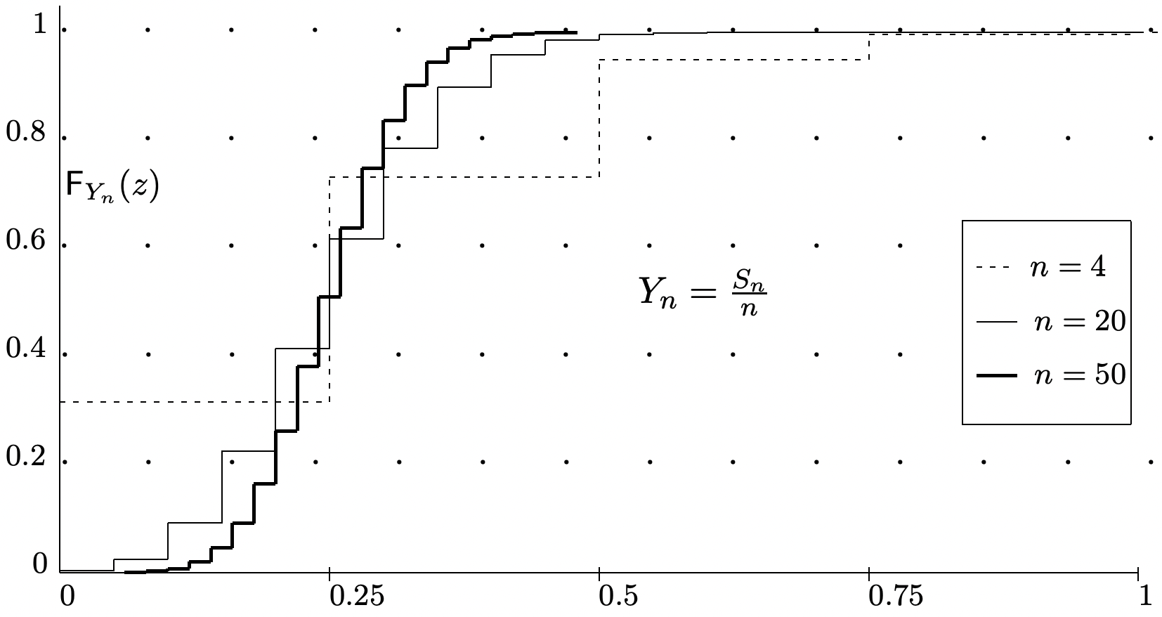
This says that the standard deviation of the sample average \(S_{n} / n\) is \(\sigma / \sqrt{n}\), which approaches 0 as \(n\) increases. Figure 1.10 illustrates this decrease in the standard deviation of \(S_{n} / n\) with increasing \(n\). In contrast, recall that Figure 1.5 illustrated how the standard deviation of \(S_{n}\) increases with \(n\). From (1.73), we see that

\[\lim _{n \rightarrow \infty} \mathrm{E}\left[\left(\frac{S_{n}}{n}-\bar{X}\right)^{2}\right]^{\}}=0\label{1.74} \]

As a result, we say that \(S_{n} / n\) converges in mean square to \(\bar{X}\).

Figure 1.10: The same distribution as Figure 1.5, scaled differently to give the distribution function of the sample average \(Y_{n}\). It can be visualized that as \(n\) increases, the distribution function of \(Y_{n}\) becomes increasingly close to a unit step at the mean, 0.25, of the variables \(X\) being summed.

This convergence in mean square says that the sample average, \(S_{n} / n\), differs from the mean, \(\bar{X}\), by a random variable whose standard deviation approaches 0 with increasing \(n\). This convergence in mean square is one sense in which \(S_{n} / n\) approaches \(\bar{X}\), but the idea of a sequence of rv’s (i.e., a sequence of functions) approaching a constant is clearly much more involved than a sequence of numbers approaching a constant. The laws of large numbers bring out this central idea in a more fundamental, and usually more useful, way. We start the development by applying the Chebyshev inequality \ref{1.56} to the sample average,

\[\operatorname{Pr}\left\{\left|\frac{S_{n}}{n}-\bar{X}\right|>\epsilon\right\}^{\}} \leq \frac{\sigma^{2}}{n \epsilon^{2}}\label{1.75} \]

This is an upper bound on the probability that \(S_{n} / n\) differs by more than \(\epsilon\) from its mean, \(\bar{X}\). This is illustrated in Figure 1.10 which shows the distribution function of \(S_{n} / n\) for various \(n\). The figure suggests that \(\lim _{n \rightarrow \infty} \mathrm{F}_{S_{n} / n}(y)=0\) for all \(y<\bar{X}\) and \(\lim _{n \rightarrow \infty} \mathrm{F}_{S_{n} / n}(y)=1\) for all \(y>\bar{X}\). This is stated more cleanly in the following weak law of large numbers, abbreviated WLLN

Theorem 1.5.1 (WLLN with finite variance). For each integer \(n \geq 1\), let \(S_{n}=X_{1}+\dots+X_n\) be the sum of \(n\) IID rv’s with a finite variance. Then the following holds:

\[\lim _{n \rightarrow \infty} \operatorname{Pr}\left\{\left|\frac{S_{n}}{n}-\bar{X}\right|>\epsilon\right\}^{\}}=0 \quad \text { for every } \epsilon>0\label{1.76} \]

Proof: For every \(\epsilon>0\), \(\operatorname{Pr}\left\{\left|S_{n} / n-\bar{X}\right|>\epsilon\right.\) is bounded between 0 and \(\sigma^{2} / n \epsilon^{2}\). Since the upper bound goes to 0 with increasing \(n\), the theorem is proved.

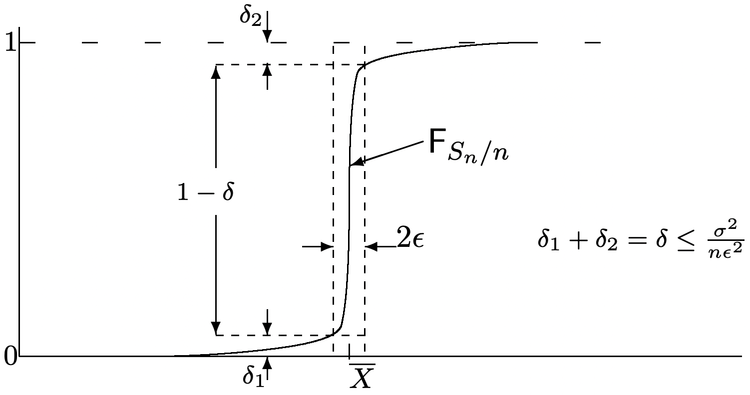
Discussion: The algebraic proof above is both simple and rigorous. However, the geometric argument in Figure 1.11 probably provides more intuition about how the limit takes place. It is important to understand both.

Figure 1.11: Approximation of the distribution function \(\mathrm{F}_{S_{n} / n}\) of a sample average by a step function at the mean: From (1.75), the probability \(\delta\) that \(S_{n} / n\) differs from \(\bar{X}\) by more than \(\epsilon\) (i.e., \(\operatorname{Pr}\left\{\left|S_{n} / n-\bar{X}\right| \geq \epsilon\right.\)) is at most \(\sigma^{2} / n \epsilon^{2}\). The complementary event, where \(\left|S_{n} / n-\bar{X}\right|<\epsilon\), has probability \(1-\delta \geq 1-\sigma^{2} / n \epsilon^{2}\). This means that we can construct a rectangle of width \(2 \epsilon\) centered on \(\bar{X}\) and of height \(1-\delta\) such that \(\mathrm{F}_{S_{n} / n}\) enters the rectangle at the lower left (say at \(\left(\bar{X}-\epsilon, \delta_{1}\right)\)) and exits at the upper right, say at \(\left(\bar{X}+\epsilon, 1-\delta_{2}\right)\)). Now visualize increasing \(n\) while holding \(\epsilon\) fixed. In the limit, \(1-\delta \rightarrow 1\) so \(\operatorname{Pr}\left\{\left|S_{n} / n-\bar{X}\right| \geq \epsilon \quad \rightarrow 0\right.\). Since this is true for every \(\epsilon>0\) (usually with slower convergence as \(\epsilon\) gets smaller), \(\mathrm{F}_{S_{n} / n}(y)\) approaches 0 for every \(y<\bar{X}\) and approaches 1 for every \(y>\bar{X}\), i.e., \(\mathrm{F}_{S_{n} / n}\) approaches a unit step at \(\bar{X}\). Note that there are two ‘fudge factors’ here, \(\epsilon\) and \(\delta\) and, since we are approximating an entire distribution function, neither can be omitted, except by directly going to a limit as \(n \rightarrow \infty\).

We refer to \ref{1.76} as saying that \(S_{n} / n\) converges to \(\bar{X}\) in probability. To make sense out of this, we should view \(\bar{X}\) as a deterministic random variable, i.e., a rv that takes the value \(\bar{X}\) for each sample point of the space. Then \ref{1.76} says that the probability that the absolute difference, \(\left|S_{n} / n-\bar{X}\right|\), exceeds any given \(\epsilon>0\) goes to 0 as \(n \rightarrow \infty\).³¹

One should ask at this point what \ref{1.76} adds to the more specific bound in (1.75). In particular \ref{1.75} provides an upper bound on the rate of convergence for the limit in (1.76). The answer is that \ref{1.76} remains valid when the theorem is generalized. For variables that are not IID or have an infinite variance, \ref{1.75} is no longer necessarily valid. In some situations, as we see later, it is valuable to know that \ref{1.76} holds, even if the rate of convergence is extremely slow or unknown.

One diculty with the bound in \ref{1.75} is that it is extremely loose in most cases. If \(S_{n} / n\) actually approached \(\bar{X}\) this slowly, the weak law of large numbers would often be more a mathematical curiosity than a highly useful result. If we assume that the MGF of X exists in an open interval around 0, then \ref{1.75} can be strengthened considerably. Recall from \ref{1.64} and \ref{1.65} that for any \(\epsilon>0\),

\[\operatorname{Pr}\left\{S_{n} / n-\bar{X} \geq \epsilon \quad \leq \exp \left(n \mu_{X}(\bar{X}+\epsilon)\right)\right.\label{1.77} \]

\[\operatorname{Pr}\left\{S_{n} / n-\bar{X} \leq-\epsilon \leq \exp \left(n \mu_{X}(\bar{X}-\epsilon)\right)\right.\label{1.78} \]

where from Lemma 1.4.1, \(\mu_{X}(a)=\inf _{r}\left\{\gamma_{X}(r)-r a\right\}<0\) for \(a \neq \bar{X}\). Thus, for any \(\epsilon>0\),

\[\operatorname{Pr}\left\{\left|S_{n} / n-\bar{X}\right| \geq \epsilon \leq \exp \left[n \mu_{X}(\bar{X}+\epsilon)\right]+\exp \left[n \mu_{X}(\bar{X}-\epsilon)\right]\right.\label{1.79} \]

The bound here, for any given \(\epsilon>0\), decreases geometrically in \(n\) rather than harmonically. In terms of Figure 1.11, the height of the rectangle must approach 1 at least geometrically in \(n\).

Relative frequency

We next show that \ref{1.76} can be applied to the relative frequency of an event as well as to the sample average of a random variable. Suppose that \(A\) is some event in a single experiment, and that the experiment is independently repeated \(n\) times. Then, in the probability model for the \(n\) repetitions, let \(A_{i}\) be the event that \(A\) occurs at the \(i \text { th }\) trial, \(1 \leq i \leq n\). The events \(A_{1}, A_{2}, \ldots, A_{n}\) are then IID.

If we let \(\mathbb{I}_{A_{i}}\) be the indicator rv for A on the \(i \text { th }\) trial, then the rv \(S_{n}=\mathbb{I}_{A_{1}}+\mathbb{I}_{A_{2}}+\cdots+\mathbb{I}_{A_{n}}\) is the number of occurrences of \(A\) over the \(n\) trials. It follows that

\[\text { relative frequency of } A=\frac{S_{n}}{n}=\frac{\sum_{i=1}^{n} \mathbb{I}_{A_{i}}}{n} \text { . }\label{1.80} \]

Thus the relative frequency of \(A\) is the sample average of the binary rv’s \(\mathbb{I}_{A_{i}}\), and everything we know about the sum of IID rv’s applies equally to the relative frequency of an event. In fact, everything we know about the sums of IID binary rv’s applies to relative frequency.

central limit theorem

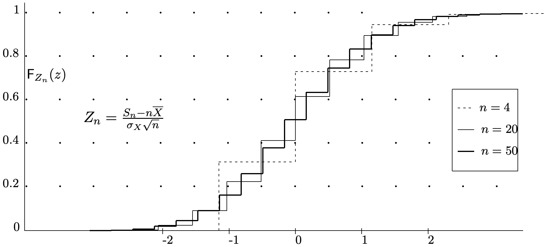
The weak law of large numbers says that with high probability, \(S_{n} / n\) is close to \(\bar{X}\) for large \(n\), but it establishes this via an upper bound on the tail probabilities rather than an estimate of what \(\mathrm{F}_{S_{n} / n}\) looks like. If we look at the shape of \(\mathrm{F}_{S_{n} / n}\) for various values of \(n\) in the example of Figure 1.10, we see that the function \(\mathrm{F}_{S_{n} / n}\) becomes increasingly compressed around \(\bar{X}\) as \(n\) increases (in fact, this is the essence of what the weak law is saying). If we normalize the random variable \(S_{n} / n\) to 0 mean and unit variance, we get a normalized rv, \(Z_{n}=\left(S_{n} / n-\bar{X}\right) \sqrt{n} / \sigma\). The distribution function of \(Z_{n}\) is illustrated in Figure 1.12 for the same underlying \(X\) as used for \(S_{n} / n\) in Figure 1.10. The curves in the two figures are the same except that each curve has been horizontally scaled by \(\sqrt{n}\) in Figure 1.12.

Inspection of Figure 1.12 shows that the normalized distribution functions there seem to be approaching a limiting distribution. The critically important central limit theorem states that there is indeed such a limit, and it is the normalized Gaussian distribution function.

Figure 1.12: The same distribution functions as Figure 1.5 normalized to 0 mean and unit standard deviation, i.e., the distribution functions of \(Z_{n}=\left(S_{n} / n-\bar{X}\right) \frac{\sqrt{n}}{\sigma_{X}}\) for \(n\)=4, 20, 50. Note that as \(n\) increases, the distribution function of \(Z_{n}\) slowly starts to resemble the normal distribution function.

Theorem 1.5.2 (Central limit theorem (CLT)). Let \(X_{1}, X_{2}, \ldots\) be IID rv’s with finite mean \(\bar{X}\) and finite variance \(\sigma^{2}\). Then for every real number \(z\),

\[\lim _{n \rightarrow \infty} \operatorname{Pr}\left\{\frac{S_{n}-n \bar{X}}{\sigma \sqrt{n}} \leq z\right\}^{\}}=\Phi(z)\label{1.81} \]

where \(\Phi(z)\) is the normal distribution function, i.e., the Gaussian distribution with mean 0 and variance 1,

\(\Phi(z)=\int_{-\infty}^{\}z} \frac{1}{\sqrt{2 \pi}} \exp \left(-\frac{y^{2}}{2}\right) d y\)

Discussion: The rv’s \(Z_{n}=\left(S_{n}-n \bar{X}\right) /(\sigma \sqrt{n})\) for each \(n \geq 1\) on the left side of \ref{1.81} each have mean 0 and variance 1. The central limit theorem (CLT), as expressed in (1.81), says that the sequence of distribution functions, \(\mathrm{F}_{Z_{1}}(z)\), \(\mathrm{F}_{Z_{2}}(z), \ldots\) converges at each value of \(z\) to \(\Phi(z)\) as \(n \rightarrow \infty\). In other words, \(\lim _{n \rightarrow \infty} \mathrm{F}_{Z_{n}}(z)=\Phi(z)\) for each \(z \in \mathbb{R}\). This is called convergence in distribution, since it is the sequence of distribution functions, rather than the sequence of rv’s that is converging. The theorem is illustrated by Figure 1.12.

The reason why the word central appears in the CLT can be seen by rewriting \ref{1.81} as

\[\lim _{n \rightarrow \infty} \operatorname{Pr}\left\{\frac{S_{n}}{n}-\bar{X} \leq \frac{\sigma z}{\sqrt{n}}\right\}^{\}}=\Phi(z), \label{1.82} \]

Asymptotically, then, we are looking at a sequence of sample averages that differ from the mean by a quantity going to 0 with \(n\) as \(1 / \sqrt{n}\), i.e., by sample averages very close to the mean for large \(n\). This should be contrasted with the optimized Chernoff bound in \ref{1.64} and \ref{1.65} which look at a sequence of sample averages that differ from the mean by a constant amount for large \(n\). These latter results are exponentially decreasing in \(n\) and are known as large deviation results.

The CLT says nothing about speed of convergence to the normal distribution. The BerryEsseen theorem (see, for example, Feller, [8]) provides some guidance about this for cases in which the third central moment \(\left.\mathrm{E}\left[|X-\bar{X}|^{3}\right]\right\}\) exists. This theorem states that

\[\left|\operatorname{Pr}\left\{\frac{\left.S_{n}-n \bar{X}\right)}{\sigma \sqrt{n}} \leq z\right\}-\Phi(z)\right| \leq \frac{\left.C \mathrm{E}\left[|X-\bar{X}|^{3}\right]\right\}}{\sigma^{3} \sqrt{n}}\label{1.83} \]

where \(C\) can be upper bounded by 0.766. We will come back shortly to discuss convergence in greater detail.

The CLT helps explain why Gaussian rv’s play such a central role in probability theory. In fact, many of the cookbook formulas of elementary statistics are based on the tacit assumption that the underlying variables are Gaussian, and the CLT helps explain why these formulas often give reasonable results.

One should be careful to avoid reading more into the CLT than it says. For example, the normalized sum, \(\left(S_{n}-n \bar{X}\right) / \sigma \sqrt{n}\) need not have a density that is approximately Gaussian. In fact, if the underlying variables are discrete, the normalized sum is discrete and has no density. The PMF of the normalized sum can have very detailed fine structure; this does not disappear as \(n\) increases, but becomes “integrated out” in the distribution function.

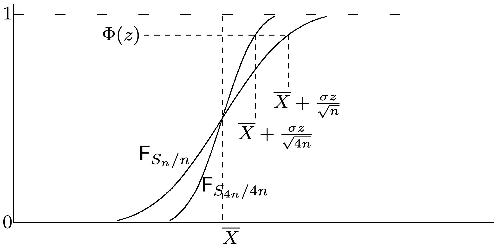
The CLT tell us quite a bit about how \(\mathrm{F}_{S_{n} / n}\) converges to a step function at \(\bar{X}\). To see this, rewrite \ref{1.81} in the form

\[\lim _{n \rightarrow \infty} \operatorname{Pr}\left\{\frac{S_{n}}{n}-\bar{X} \leq \frac{\sigma z}{\sqrt{n}}\right\}^{\}}=\Phi(z)\label{1.84} \]

This is illustrated in Figure 1.13 where we have used \(\Phi(z)\) as an approximation for the probability on the left.

A proof of the CLT requires mathematical tools that will not be needed subsequently. Thus we give a proof only for the binomial case. Feller ([7] and [8]) gives a thorough and careful exposition and proof of several versions of the CLT including those here.³²

Proof*³³ of Theorem 1.5.2 (binomial case): We first establish a somewhat simpler result which uses finite limits on both sides of \(\left(S_{n}-n \bar{X}\right) / \sigma \sqrt{n}\), i.e., we show that for any finite \(y<z\),

\[\left.\lim _{n \rightarrow \infty} \operatorname{Pr}\left\{y<\frac{S_{n}-n \bar{X}}{\sigma \sqrt{n}} \leq z\right\}^{\}}=\int_{y}^{\}z} \frac{1}{\sqrt{2 \pi}} \exp \left(\frac{-u^{2}}{2}\right)\right\} d u\label{1.85} \]

Figure 1.13: Approximation of the distribution function \(\mathrm{F}_{S_{n} / n}\) of a sample average by a Gaussian distribution of the same mean and variance. Whenever \(n\) is increased by a factor of 4, the curve is horizontally scaled inward toward \(\bar{X}\) by a factor of 2. The CLT says both that these curves are scaled horizontally as \(1 / \sqrt{n}\) and also that they are better approximated by the Gaussian of the given mean and variance as \(n\) increases.

The probability on the left of \ref{1.85} can be rewritten as

\[\begin{gathered}
\operatorname{Pr}\left\{y<\frac{S_{n}-n \bar{X}}{\sigma \sqrt{n}} \leq z\right\}^{\}}=\operatorname{Pr}\left\{\frac{\sigma y}{\sqrt{n}}<\frac{S_{n}}{n}-\bar{X} \leq \frac{\sigma z}{\sqrt{n}}\right\}^{\}} \\
=\sum_{k} \mathrm{p}_{S_{n}}(k) \text { for } \frac{\sigma y}{\sqrt{n}}<\frac{k}{n}-p \leq \frac{\sigma z}{\sqrt{n}}
\end{gathered}\label{1.86} \]

Let \(\tilde{p}=k / n\), \(\tilde{q}=1-\tilde{p}\), and \(\epsilon(k, n)=\tilde{p}-p\). We abbreviate \(\epsilon(k, n)\) as \(\epsilon\) where \(k\) and \(n\) are clear from the context. From (1.23), we can express \(\mathrm{p}_{S_{n}}(k)\) as

\[\begin{aligned}
\mathrm{p}_{S_{n}}(k) & \sim \frac{1}{\sqrt{2 \pi n \tilde{p} \tilde{q}}} \exp n[\tilde{p} \ln (p / \tilde{p})+\tilde{q} \ln (q / \tilde{q})] \\
&=\frac{1}{\sqrt{2 \pi n(p+\epsilon)(q-\epsilon)}} \exp \left[-n(p+\epsilon) \ln \left(1+\frac{\epsilon}{p}\right)-n(q-\epsilon) \ln \left(1-\frac{\epsilon}{q}\right)\right]^{\}} \\
&=\frac{1}{\sqrt{2 \pi n(p+\epsilon)(q-\epsilon)}} \exp \left[-n\left(\frac{\epsilon^{2}}{2 p}-\frac{\epsilon^{3}}{6 p^{2}}+\cdots+\frac{\epsilon^{2}}{2 q}+\frac{\epsilon^{3}}{6 q^{2}} \cdots\right)\right] .
\end{aligned}\label{1.87} \]

where we have used the power series expansion, \(\ln (1+u)=u-u^{2} / 2+u^{3} / 3 \cdots\) From (1.86), \(\sigma y / \sqrt{n}<p+\epsilon(k, n) \leq \sigma z / \sqrt{n}\), so the omitted terms in \ref{1.87} go to 0 uniformly over the range of \(k\) in (1.86). The term \((p+\epsilon)(q-\epsilon)\) also converges (uniformly in \(k\)) to \(pq\) as \(n \rightarrow \infty\). Thus

\[\begin{aligned}
\mathrm{p}_{S_{n}}(k) &\sim \frac{1}{\sqrt{2 \pi n p q}} \exp \left[-n\left(\frac{\epsilon^{2}}{2 p}+\frac{\epsilon^{2}}{2 q}\right)\right]^{\}} \\
&=\frac{1}{\sqrt{2 \pi n p q}} \exp \left[\frac{-n \epsilon^{2}}{2 p q}\right]^{\}} \\
&=\frac{1}{\sqrt{2 \pi n p q}} \exp \left[\frac{-u^{2}(k, n)}{2}\right]^{\}} \quad \text { where } u(k, n)=\frac{k-n p}{\sqrt{p q n}} .
\end{aligned}\label{1.88} \]

Since the ratio of the right to left side in \ref{1.88} approaches 1 uniformly in \(k\) over the given range of \(k\),

\[\sum_{k} \mathrm{p}_{S_{n}}(k) \sim \sum\ _{k}^{\}}\frac{1}{\sqrt{2 \pi n p q}} \exp \left[\frac{-u^{2}(k, n)}{2}\right]\label{1.89} \]

Since \(u(k, n)\) increases in increments of \(1 / \sqrt{p q n}\), we can view the sum on the right above as a Riemann sum approximating (1.85). Since the terms of the sum get closer as \(n \rightarrow \infty\), and since the Riemann integral exists, \ref{1.85} must be satisfied in the limit.

To complete the proof, note from the Chebyshev inequality that

\(\operatorname{Pr}\left\{\left|S_{n}-\bar{X}\right| \geq \frac{\sigma|y|}{\sqrt{n}}\right\}^{\}} \leq \frac{1}{y^{2}},\)

and thus

\(\operatorname{Pr}\left\{y<\frac{S_{n}-n \bar{X}}{\sigma \sqrt{n}} \leq z\right\}^{\}} \leq \operatorname{Pr}\left\{\frac{S_{n}-n \bar{X}}{\sigma \sqrt{n}} \leq z\right\}^{\}} \leq \frac{1}{y^{2}}+\operatorname{Pr}\left\{y<\frac{S_{n}-n \bar{X}}{\sigma \sqrt{n}} \leq z\right\}^{\}}\)

Choosing \(y=-n^{1 / 4}\), we see that \(1 / y^{2} \rightarrow 0\) as \(n \rightarrow \infty\). Also \(n \epsilon^{3}(k, n)\) in \ref{1.87} goes to 0 as \(n \rightarrow \infty\) for all \((k, n)\) satisfying \ref{1.86} with \(y=-n^{1 / 4}\). Taking the limit as \(n \rightarrow \infty\) then proves the theorem.

If we trace through the various approximations in the above proof, we see that the error in \(\mathrm{p}_{S_{n}}(k)\) goes to 0 as \(1 / n\). This is faster than the \(1 / \sqrt{n}\) bound in the Berry-Esseen theorem. If we look at Figure 1.3, however, we see that the distribution function of \(S_{n} / n\) contains steps of order \(1 / \sqrt{n}\). These vertical steps cause the binomial result here to have the same slow \(1 / \sqrt{n}\) convergence as the general Berry-Esseen bound. It turns out that if we evaluate the distribution function only at the midpoints between these steps, i.e., at \(z=(k+1 / 2-n p) / \sigma \sqrt{n}\), then the convergence in the distribution function is of order \(1 / n\).

Since the CLT provides such explicit information about the convergence of \(S_{n} / n\) to \(\bar{X}\), it is reasonable to ask why the weak law of large numbers (WLLN) is so important. The first reason is that the WLLN is so simple that it can be used to give clear insights to situations where the CLT could confuse the issue. A second reason is that the CLT requires a variance, where as we see next, the WLLN does not. A third reason is that the WLLN can be extended to many situations in which the variables are not independent and/or not identically distributed.³⁴ A final reason is that the WLLN provides an upper bound on the tails of \(\mathrm{F}_{S_{n} / n}\), whereas the CLT provides only an approximation.

Weak law with an infinite variance

We now establish the WLLN without assuming a finite variance.

Theorem 1.5.3 (WLLN). For each integer \(n \geq 1\), let \(S_{n}=X_{1}+\cdots+X_{n}\) where \(X_{1}, X_{2}, \ldots\) are IID rv’s satisfying \(\mathrm{E}[|X|]<\infty\). Then for any \(\epsilon>0\),

\[\lim _{n \rightarrow \infty} \operatorname{Pr}\left\{\left|\frac{S_{n}}{n}-\mathrm{E}[X]\right|>\epsilon\right\}^{\}}=0\label{1.90} \]

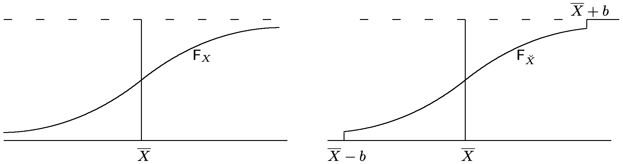
Proof:³⁵ We use a truncation argument; such arguments are used frequently in dealing with rv’s that have infinite variance. The underlying idea in these arguments is important, but some less important details are treated in Exercise 1.35. Let \(b\) be a positive number (which we later take to be increasing with \(n\)), and for each variable \(X_{i}\), define a new rv \(\breve{X}_{i}\) (see Figure 1.14) by

\[\breve{X}_{i}= \begin{cases}X_{i} & \text { for } \quad \mathrm{E}[X]-b \leq X_{i} \leq \mathrm{E}[X]+b \\ \}_{\mathrm{E}}[X]+b & \text { for } \quad X_{i}>\mathrm{E}[X]+b \\ \} \mathrm{E}[X]-b & \text { for } \quad X_{i}<\mathrm{E}[X]-b\end{cases}\label{1.91} \]

Figure 1.14: The truncated rv \(\breve{X}\) for a given rv X has a distribution function which is truncated at \(\bar{X} \pm b\).

The truncated variables \(\breve{X}_{i}\) are IID and, because of the truncation, must have a finite second moment. Thus the WLLN applies to the sample average \(\breve{S}_{n}=\breve{X}_{1}+\cdots \breve{X}_{n}\). More particularly, using the Chebshev inequality in the form of \ref{1.75} on \(\breve{S}_{n} / n\), we get

\(\operatorname{Pr}\left\{\left|\frac{\breve{S}_{n}}{n}-\mathrm{E}[\breve{X}]\right|>\frac{\epsilon}{2}\right\}^{\}} \leq \frac{4 \sigma_{\breve{X}}^{2}}{n \epsilon^{2}} \leq \frac{8 b \mathrm{E}[|X|]}{n \epsilon^{2}}\),

where Exercise 1.35 demonstrates the final inequality. Exercise 1.35 also shows that \(\mathrm{E}[\breve{X}]\}\) approaches \(\mathrm{E}[X]\) as \(b \rightarrow \infty\) and thus that

\[\operatorname{Pr}\left\{\left|\frac{\breve{S}_{n}}{n}-\mathrm{E}[X]\right|>\epsilon\right\}^{\}} \leq \frac{8 b \mathrm{E}[|X|]}{n \epsilon^{2}},\label{1.92} \]

for all suciently large \(b\). This bound also applies to \(S_{n} / n\) in the case where \(S_{n}=\breve{S}_{n}\), so we have the following bound (see Exercise 1.35 for further details):

\[\operatorname{Pr}\left\{\left|\frac{S_{n}}{n}-\mathrm{E}[X]\right|>\epsilon\right\}^{\}} \leq \operatorname{Pr}\left\{\left|\frac{\breve{S}_{n}}{n}-\mathrm{E}[X]\right|>\epsilon\right\}+\operatorname{Pr}\left\{S_{n} \neq \breve{S}_{n}\right\}.\label{1.93} \]

The original sum \(S_{n}\) is the same as \(\breve{S}_{n}\) unless one of the \(X_{i}\) has an outage, i.e., \(\left|X_{i}-\bar{X}\right|>b\). Thus, using the union bound, \(\operatorname{Pr}\left\{S_{n} \neq \breve{S}_{n}\right\}^{\}} \leq n \operatorname{Pr}\left\{\left|X_{i}-\bar{X}\right|>b\right.\). Substituting this and \ref{1.92} into (1.93),

\[\operatorname{Pr}\left\{\left|\frac{S_{n}}{n}-\mathrm{E}[X]\right|>\epsilon\right\}^{\}}{\leq} \frac{8 b \mathrm{E}[|X|]}{n \epsilon^{2}}+\frac{n}{b}[b \operatorname{Pr}\{|X-\mathrm{E}[X]|>b\}]. \label{1.94} \]

We now show that for any \(\epsilon>0\) and \(\delta>0\), \(\operatorname{Pr}\left\{\left|S_{n} / n-\bar{X}\right| \geq \epsilon \leq \delta\right.\) for all suciently large \(n\). We do this, for given \(\epsilon, \delta\), by choosing \(b(n)\) for each \(n\) so that the first term in \ref{1.94} is equal to \(\delta / 2\). Thus \(b(n)=n \delta \epsilon^{2} / 16 \mathrm{E}[|X|]\). This means that \(n / b(n)\) in the second term is independent of \(n\). Now from (1.55), \(\lim _{b \rightarrow \infty} b \operatorname{Pr}\{|X-\bar{X}|>b=0\), so by choosing \(b(n)\) suciently large (and thus \(n\) suciently large), the second term in \ref{1.94} is also at most \(\delta / 2\).

Convergence of random variables

This section has now developed a number of results about how the sequence of sample averages, \(\left\{S_{n} / n ; n \geq 1\right\}\) for a sequence of IID rv’s \(\left\{X_{i} ; i \geq 1\right\}\) approach the mean \(\bar{X}\). In the case of the CLT, the limiting distribution around the mean is also specified to be Gaussian. At the outermost intuitive level, i.e., at the level most useful when first looking at some very complicated set of issues, viewing the limit of the sample averages as being essentially equal to the mean is highly appropriate.

At the next intuitive level down, the meaning of the word essentially becomes important and thus involves the details of the above laws. All of the results involve how the rv’s \(S_{n} / n\) change with \(n\) and become better and better approximated by \(\bar{X}\). When we talk about a sequence of rv’s (namely a sequence of functions on the sample space) being approximated by a rv or numerical constant, we are talking about some kind of convergence, but it clearly is not as simple as a sequence of real numbers (such as \(1 / n\) for example) converging to some given number (0 for example).

The purpose of this section, is to give names and definitions to these various forms of convergence. This will give us increased understanding of the laws of large numbers already developed, but, equally important, It will allow us to develop another law of large numbers called the strong law of large numbers (SLLN). Finally, it will put us in a position to use these convergence results later for sequences of rv’s other than the sample averages of IID rv’s.

We discuss four types of convergence in what follows, convergence in distribution, in probability, in mean square, and with probability 1. For the first three, we first recall the type of large-number result with that type of convergence and then give the general definition.

For convergence with probability 1 (WP1), we first define this type of convergence and then provide some understanding of what it means. This will then be used in Chapter 4 to state and prove the SLLN.

We start with the central limit theorem, which, from \ref{1.81} says

\(\lim _{n \rightarrow \infty} \operatorname{Pr}\left\{\frac{S_{n}-n \bar{X}}{\sqrt{n} \sigma} \leq z\right\}^{\}}=\int_{-\infty}^{\}z} \frac{1}{\sqrt{2 \pi}} \exp \left(\frac{-x^{2}}{2}\right)^{\}} d x \quad \text { for every } z \in \mathbb{R}\)

This is illustrated in Figure 1.12 and says that the sequence (in \(n\)) of distribution functions \(\operatorname{Pr}\left\{\frac{S_{n}-n \bar{X}}{\sqrt{n} \sigma} \leq z\right\}^{\}}\) converges at every \(z\) to the normal distribution function at \(z\). This is an example of convergence in distribution.

Definition 1.5.1. A sequence of random variables, \(Z_{1}, Z_{2}, \ldots\) converges in distribution to a random variable \(Z\) if \(\lim _{n \rightarrow \infty} \mathrm{F}_{Z_{n}}(z)=\mathrm{F}_{Z}(z)\) at each \(z\) for which \(\mathrm{F}_{Z}(z)\) is continuous.

For the CLT example, the rv’s that converge in distribution are \(\left\{\frac{S_{n}-n \bar{X}}{\sqrt{n} \sigma} ; n \geq 1\right\}\), and they n converge in distribution to the normal Gaussian rv.

Convergence in distribution does not say that the rv’s themselves converge in any reasonable sense, but only that their distribution functions converge. For example, let \(Y_{1}, Y_{2}, \ldots\), be IID rv’s, each with the distribution function \(\mathrm{F}_{Y}\). For each \(n \geq 1\), if we let let \(Z_{n}=Y_{n}+1 / n\), then it is easy to see that \(\left\{Z_{n} ; n \geq 1\right\}\) converges in distribution to \(Y\). However (assuming \(Y\) has variance \(\sigma_{Y}^{2}\) and is independent of each \(Z_{n}\)), we see that \(Z_{n}-Y\) has variance \(2 \sigma_{Y}^{2}\). Thus \(Z_{n}\) does not get close to \(Y\) as \(n \rightarrow \infty\) in any reasonable sense, and \(Z_{n}-Z_{m}\) does not get small as \(n\) and \(m\) both get large.³⁶ As an even more trivial example, the sequence \(\left\{Y_{n} n \geq 1\right\}\) converges in distribution to \(Y\).

For the CLT, it is the rv’s \(\frac{S_{n}-n \bar{X}}{\sqrt{n} \sigma}\) that converge in distribution to the normal. As shown in Exercise 1.38, however, the rv \(\frac{S_{n}-n \bar{X}}{\sqrt{n} \sigma}-\frac{S_{2 n}-2 n \bar{X}}{\sqrt{2 n} \sigma}\) is not close to 0 in any reasonable sense, even though the two terms have distribution functions that are very close for large \(n\).

For the next type of convergence of rv’s, the WLLN, in the form of (1.90), says that

\(\lim _{n \rightarrow \infty} \operatorname{Pr}\left\{\left|\frac{S_{n}}{n}-\bar{X}\right|>\epsilon\right\}^{\}}=0 \quad \text { for every } \epsilon>0\)

This is an example of convergence in probability, as defined below:

Definition 1.5.2. A sequence of random variables \(Z_{1}, Z_{2}, \ldots\), converges in probability to a rv \(Z\) if \(\lim _{n \rightarrow \infty} \operatorname{Pr}\left\{\left|Z_{n}-Z\right|>\epsilon\right\}=0\) for every \(\epsilon>0\).

For the WLLN example, \(Z_{n}\) in the definition is the relative frequency \(S _{n} / n\) and \(Z\) is the constant rv \(\bar{X}\). It is probably simpler and more intuitive in thinking about convergence of rv’s to think of the sequence of rv’s \(\left\{Y_{n}=Z_{n}-Z ; n \geq 1\right\}\) as converging to 0 in some sense.³⁷ As illustrated in Figure 1.10, convergence in probability means that \(\left\{Y_{n} ; n \geq 1\right\}\) converges in distribution to a unit step function at 0.

An equivalent statement, as illustrated in Figure 1.11, is that \(\left\{Y_{n} ; n \geq 1\right\}\) converges in probability to 0 if \(\lim _{n \rightarrow \infty} \mathrm{F}_{Y_{n}}(y)=0\) for all \(y<0\) and \(\lim _{n \rightarrow \infty} \mathrm{F}_{Y_{n}}(y)=1\) for all \(y>0\). This shows that convergence in probability is a special case of convergence in distribution, since with convergence in probability, the sequence \(F_{Y_{n}}\) of distribution functions converges to a unit step at 0. Note that \(\lim _{n \rightarrow \infty} \mathrm{F}_{Y_{n}}(y)\) is not specified at \(y = 0\). However, the step function is not continuous at 0, so the limit there need not be specified for convergence in distribution.

Convergence in probability says quite a bit more than convergence in distribution. As an important example of this, consider the difference \(Y_{n}-Y_{m}\) for \(n\) and \(m\) both large. If \(\{Y_{n} ; n \geq1\}\) converges in probability to 0, then \(Y_{n}\) and \(Y_{m}\) are both close to 0 with high probability for large \(n\) and \(m\), and thus close to each other. More precisely, \(\lim _{m \rightarrow \infty, n \rightarrow \infty} \operatorname{Pr}\left\{\left|Y_{n}-Y_{m}\right|>\epsilon\right\}=0\) for every \(\epsilon>0\). If the sequence \(\left\{Y_{n} ; n \geq 1\right\}\) merely converges in distribution to some arbitrary distribution, then, as we saw, \(Z_{n}-Z_{m}\) can be large with high probability, even when \(n\) and \(m\) are large. Another example of this is given in Exercise 1.38.

It appears paradoxical that the CLT is more explicit about the convergence of \(S_{n} / n\) to \(\bar{X}\) than the weak law, but it corresponds to a weaker type of convergence. The resolution of this paradox is that the sequence of rv’s in the CLT is \(\left\{\frac{S_{n}-n \bar{X}}{\sqrt{n} \sigma} ; n \geq 1\right\}\). The presence of \(\sqrt{n}\) in the denominator of this sequence provides much more detailed information about how \(S_{n} / n\) approaches \(\bar{X}\) with increasing \(n\) than the limiting unit step of \(\mathrm{F}_{S_{n} / n}\) itself. For example, it is easy to see from the CLT that \(\lim _{n \rightarrow \infty} \mathrm{F}_{S_{n} / n}(\bar{X})=1 / 2\), which can not be derived directly from the weak law.

Yet another kind of convergence is convergence in mean square (MS). An example of this, for the sample average \(S_{n} / n\) of IID rv’s with a variance, is given in (1.74), repeated below:

\(\lim _{n \rightarrow \infty} \mathrm{E}\left[\left(\frac{S_{n}}{n}-\bar{X}\right)^{2}\right]^{\}}=0\)

The general definition is as follows:

Definition 1.5.3. A sequence of rv’s \(Z_{1}, Z_{2}, \ldots\), converges in mean square (MS) to a rv \(Z\) if \(\left.\lim _{n \rightarrow \infty} \mathrm{E}\left[\left(Z_{n}-Z\right)^{2}\right]\right\}=0\).

Our derivation of the weak law of large numbers (Theorem 1.5.1) was essentially based on the MS convergence of (1.74). Using the same approach, Exercise 1.37 shows in general that convergence in MS implies convergence in probability. Convergence in probability does not imply MS convergence, since as shown in Theorem 1.5.3, the weak law of large numbers holds without the need for a variance.

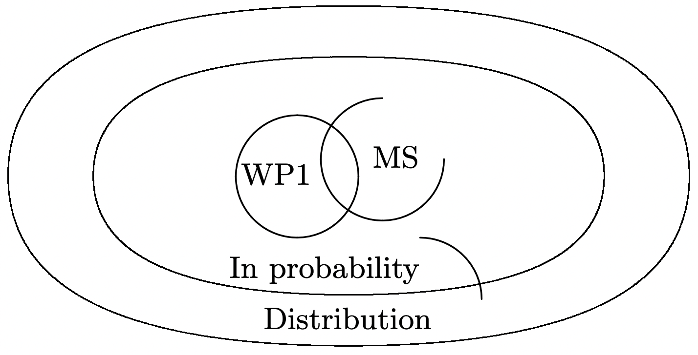
Figure 1.15 illustrates the relationship between these forms of convergence, i.e., mean square convergence implies convergence in probability, which in turn implies convergence in distribution. The figure also shows convergence with probability 1 (WP1), which is the next form of convergence to be discussed.

Figure 1.15: Relationship between different kinds of convergence: Convergence in distribution is the most general and is implied by all the others. Convergence in probability is the next most general and is implied by convergence with probability 1 (WP1) and by mean square (MS) convergence, neither of which imply the other.

Convergence with probability 1

We next define and discuss convergence with probability 1, abbreviated as convergence WP1. Convergence WP1 is often referred to as convergence a.s. (almost surely) and convergence a.e. (almost everywhere). The strong law of large numbers, which is discussed briefly in this section and further discussed and proven in various forms in Chapters 4 and 7, provides an extremely important example of convergence WP1. The general definition is as follows:

Definition 1.5.4. Let \(Z_{1}, Z_{2}, \ldots\), be a sequence of rv’s in a sample space \(\Omega\) and let \(Z\) be another rv in \(\Omega\). Then \(\left\{Z_{n} ; n \geq 1\right\}\) is defined to converge to \(Z\) with probability 1 (WP1) if

\[\operatorname{Pr}\left\{\omega \in \Omega: \lim _{n \rightarrow \infty} Z_{n}(\omega)=Z(\omega)\right\}^{\}}=1\label{1.95} \]

The condition \(\operatorname{Pr}\left\{\omega \in \Omega: \lim _{n \rightarrow \infty} Z_{n}(\omega)=Z(\omega)\right\}=1\) is often stated more compactly as \(\operatorname{Pr}\left\{\lim _{n} Z_{n}=Z\right\}=1\), and even more compactly as \(\lim _{n} Z_{n}=Z\) WP1, but the form here is the simplest for initial understanding. As discussed in Chapter 4. the SLLN says that if \(\left\{X_{i} ; i \geq 1\right\}\) are IID with \(\mathrm{E}[|X|]<\infty\), then the sequence of sample averages, \(\left\{S_{n} / n ; n \geq 1\right\}\) converges WP1 to \(\bar{X}\).

In trying to understand (1.95), note that each sample point \(\omega\) of the underlying sample space \(\Omega\) maps to a sample value \(Z_{n}(\omega)\) of each rv \(Z_{n}\), and thus maps to a sample path \(\left\{Z_{n}(\omega) ; n \geq 1\right\}\). For any given \(\omega\), such a sample path is simply a sequence of real numbers. That sequence of real numbers might converge to \(Z(\omega)\) (which is a real number for the given \(\omega\)), it might converge to something else, or it might not converge at all. Thus there is a set of \(\omega\) for which the corresponding sample path \(\left\{Z_{n}(\omega) ; n \geq 1\right\}\) converges to \(Z(\omega)\), and a second set for which the sample path converges to something else or does not converge at all. Convergence WP1 of the sequence of rv’s is thus defined to occur when the first set of sample paths above has probability 1.

For each \(\omega\), the sequence \(\left\{Z_{n}(\omega) ; n \geq 1\right\}\) is simply a sequence of real numbers, so we briefly review what the limit of such a sequence is. A sequence of real numbers \(b_{1}, b_{2}\)... is said to have a limit \(b\) if, for every \(\epsilon>0\), there is an integer \(m_{\epsilon}\) such that \(\left|b_{n}-b\right| \leq \epsilon\) for all \(n \geq m_{\epsilon}\). An equivalent statement is that \(b_{1}, b_{2}, \ldots\), has a limit \(b\) if, for every integer \(k \geq 1\), there is an integer \(m(k)\) such that \(\left|b_{n}-b\right| \leq 1 / k\) for all \(n \geq m(k)\).

Figure 1.16 illustrates this definition for those, like the author, whose eyes blur on the second or third ‘there exists’, ‘such that’, etc. in a statement. As illustrated, an important aspect of convergence of a sequence \(\left\{b_{n} ; n \geq 1\right\}\) of real numbers is that \(b_{n}\) becomes close to \(b\) for large \(n\) and stays close for all suciently large values of \(n\).

Figure 1.16: Illustration of a sequence of real numbers \(b_{1}, b_{2}, \ldots\) that converge to a number \(b\). The figure illustrates an integer \(m(1)\) such that for all \(n \geq m(1), b_{n}\) lies in the interval \(b \pm 1\). Similarly, for each \(k \geq 1\), there is an integer \(m(k)\) such that \(b_{n}\) lies in \(b \pm 1 / k\) for all \(n \geq m(k)\). Thus \(\lim _{n \rightarrow \infty} b_{n}=b\) means that for a sequence of ever tighter constraints, the kth constraint can be met for all suciently large \(n\), (i.e., all \(n \geq m(k))\). Intuitively, convergence means that the elements \(b_{1}, b_{2}, \ldots\) get close to \(b\) and stay close. The sequence of positive integers \(m(1), m(2), \ldots\) is nondecreasing, but otherwise arbitrary, depending only on the sequence \(\left\{b_{n} ; n \geq 1\right\}\). For sequences that converge very slowly, the integers \(m(1), m(2), \ldots\) are simply correspondingly larger.

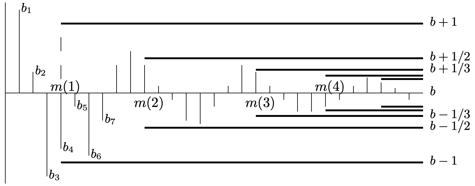
Figure 1.17 gives an example of a sequence of real numbers that does not converge. Intuitively, this sequence is close to 0 (and in fact identically equal to 0) for most large \(n\), but it doesn’t stay close

Figure 1.17: Illustration of a non-convergent sequence of real numbers \(b_{1}, b_{2}, \ldots\) The sequence is defined by \(b_{n}=3 / 4\) for \(n=1,5,25, \ldots, 5^{j}, \ldots\) for all integer \(j \geq 0\). For all other \(n, b_{n}=0\). The terms for which \(b_{n} \neq 0\) become increasingly rare as \(n \rightarrow \infty\). Note that \(b_{n} \in[1,1]\) for all \(n\), but there is no \(m(2)\) such that \(b_{n} \in\left[-\frac{1}{2}, \frac{1}{2}\right]\) for all \(n \geq m(2)\). Thus the sequence does not converge.

The following example illustrates how a sequence of rv’s can converge in probability but not converge WP1. The example also provides some clues as to why convergence WP1 is important.

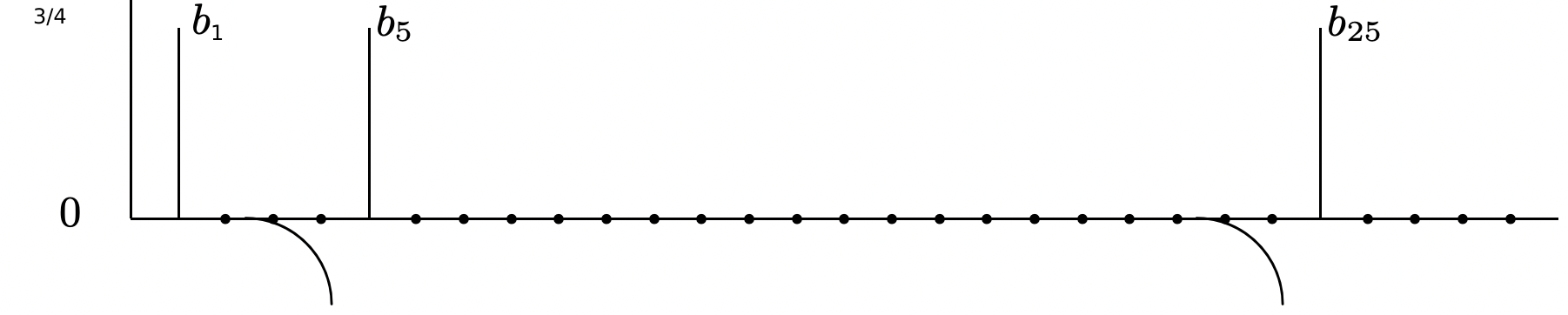
Example 1.5.1. Consider a sequence \(\left\{Z_{n} ; n \geq 1\right\}\) of rv’s for which the sample paths constitute the following slight variation of the sequence of real numbers in Figure 1.17. In particular, as illustrated in Figure 1.18, the nonzero term at \(n=5^{j}\) in Figure 1.17 is replaced by a nonzero term at a randomly chosen \(n\) in the interval \(\left[5^{j}, 5^{j+1}\right)\).

Figure 1.18: Illustration of a sample path of a sequence of rv’s \(\left\{Y_{n} ; n \geq 0\right\}\) where, for each \(j \geq 0, Y_{n}=1\) for an equiprobable choice of \(n \in\left[5^{j}, 5^{j+1}\right)\) and \(Y_{n}=0\) otherwise.

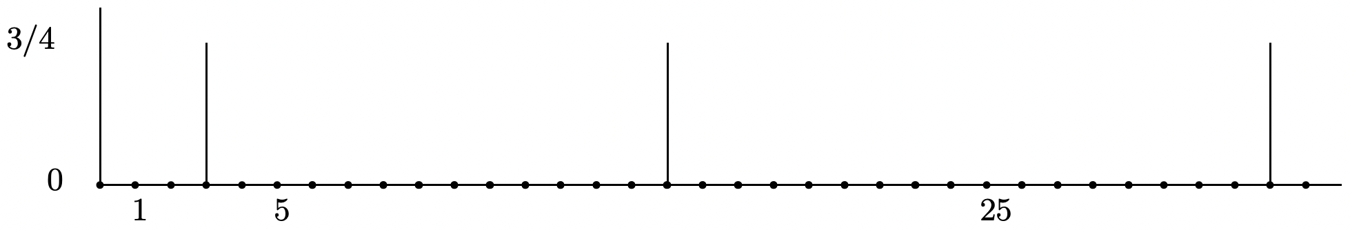
Since each sample path contains a single one in each segment \(\left[5^{j}, 5^{j+1}\right)\), and contains zero’s elsewhere, none of the sample paths converge. In other words, \(\operatorname{Pr}\left\{\omega: \lim Z_{n}(\omega)=0\right\}=0\) rather than 1. On the other hand \(\operatorname{Pr}\left\{Z_{n}=0\right\}=1-5^{-j}\) for \(5^{j} \leq n<5^{j+1}\), so \(\lim _{n \rightarrow \infty} \operatorname{Pr}\left\{Z_{n}=0\right\}=1\).

Thus this sequence of rv’s converges to 0 in probability, but does not converge to 0 WP1. This sequence also converges in mean square and (since it converges in probability) in distribution. Thus we have shown (by example) that convergence WP1 is not implied by any of the other types of convergence we have discussed. We will show in Section 4.2 that convergence WP1 does imply convergence in probability and in distribution but not in mean square (as illustrated in Figure 1.15).

The interesting point in this example is that this sequence of rv’s is not bizarre (although it is somewhat specialized to make the analysis simple). Another important point is that this definition of convergence has a long history of being accepted as the ‘useful,’ ‘natural,’ and ‘correct’ way to define convergence for a sequence of real numbers. Thus it is not surprising that convergence WP1 will turn out to be similarly useful for sequences of rv’s.

There is a price to be paid in using the concept of convergence WP1. We must then look at the entire sequence of rv’s and can no longer analyze finite \(n\)-tuples and then go to the limit as \(n \rightarrow \infty\). This requires a significant additional layer of abstraction, which involves additional mathematical precision and initial loss of intuition. For this reason we put off further discussion of convergence WP1 and the SLLN until Chapter 4 where it is needed.

---

Reference

³¹Saying this in words gives one added respect for mathematical notation, and perhaps in this case, it is preferable to simply understand the mathematical statement (1.76).

³²Many elementary texts provide ‘simple proofs,’ using transform techniques, but, among other problems, they usually indicate that the normalized sum has a density that approaches the Gaussian density, which is incorrect for all discrete rv’s.

³³This proof can be omitted without loss of continuity. However, it is an important part of achieving a thorough understanding of the CLT.

³⁴Central limit theorems also hold in many of these more general situations, but they do not hold as widely as the WLLN.

³⁵The details of this proof can be omitted without loss of continuity. However, the general structure of the truncation argument should be understood.

³⁶In fact, saying that a sequence of rv’s converges in distribution is unfortunate but standard terminology. It would be just as concise, and far less confusing, to say that a sequence of distribution functions converge rather than saying that a sequence of rv’s converge in distribution.

³⁷Definition 1.5.2 gives the impression that convergence to a rv \(Z\) is more general than convergence to a constant or convergence to 0, but converting the rv’s to \(Y_{n}=Z_{n}-Z\) makes it clear that this added generality is quite superficial.