2.1: Introduction to Poisson Processes

A Poisson process is a simple and widely used stochastic process for modeling the times at which arrivals enter a system. It is in many ways the continuous-time version of the Bernoulli process that was described in Section 1.3.5. For the Bernoulli process, the arrivals can occur only at positive integer multiples of some given increment size (often taken to be 1). Section 1.3.5 characterized the process by a sequence of IID binary random variables (rv’s), \(Y_{1}, Y_{2}, \ldots\), where \(Y_{i}=1\) indicates an arrival at increment \(i\) and \(Y_{i}=0\) otherwise. We observed (without any careful proof) that the process could also be characterized by the sequence of interarrival times. These interarrival times are geometrically distributed IID rv’s.

For the Poisson process, arrivals may occur at arbitrary positive times, and the probability of an arrival at any particular instant is 0. This means that there is no very clean way of describing a Poisson process in terms of the probability of an arrival at any given instant. It is more convenient to define a Poisson process in terms of the sequence of interarrival times, \(X_{1}, X_{2}, \ldots\), which are defined to be IID. Before doing this, we describe arrival processes in a little more detail.

Arrival processes

An arrival process is a sequence of increasing rv’s, \(0<S_{1}<S_{2}<\cdots\), where¹ \(S_{i}<S_{i+1}\) means that \(S_{i+1}-S_{i}\) is a positive rv, i.e., a rv \(X\) such that \(\mathrm{F}_{X}(0)=0\). The rv’s \(S_{1}, S_{2}, \ldots\), are called arrival epochs (the word time is somewhat overused in this subject) and represent the times at which some repeating phenomenon occurs. Note that the process starts at time 0 and that multiple arrivals can’t occur simultaneously (the phenomenon of bulk arrivals can be handled by the simple extension of associating a positive integer rv to each arrival). We will sometimes permit simultaneous arrivals or arrivals at time 0 as events of zero probability, but these can be ignored. In order to fully specify the process by the sequence \(S_{1}, S_{2}, \ldots\) of rv’s, it is necessary to specify the joint distribution of the subsequences \(S_{1}, \ldots, S_{n}\) for all \(n>1\).

Although we refer to these processes as arrival processes, they could equally well model departures from a system, or any other sequence of incidents. Although it is quite common, especially in the simulation field, to refer to incidents or arrivals as events, we shall avoid that here. The \(n\)th arrival epoch \(S_{n}\) is a rv and \(\left\{S_{n} \leq t\right\}\), for example, is an event. This would make it confusing to refer to the \(n\)th arrival itself as an event.

Figure 2.1: A sample function of an arrival process and its arrival epochs \(\left\{S_{1}, S_{2}, \ldots\right\}\), its interarrival intervals \(\left\{X_{1}, X_{2}, \ldots\right\}\), and its counting process \(\{N(t) ; t>0\}\)

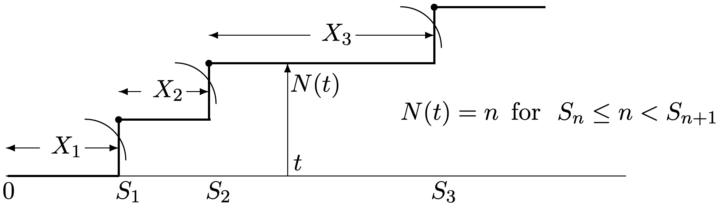
As illustrated in Figure 2.1, any arrival process can also be specified by two alternative stochastic processes. The first alternative is the sequence of interarrival times, X_{1}, X_{2}, \ldots,. These are positive rv’s defined in terms of the arrival epochs by \(X_{1}=S_{1}\) and \(X_{i}=S_{i}-S_{i-1}\) for \(i>1\). Similarly, given the \(X_{i}\), the arrival epochs \(S_{i}\) are specified as

\[S_{n}=\sum_{i=1}^{n} X_{i}\label{2.1} \]

Thus the joint distribution of \(X_{1}, \ldots, X_{n}\) for all \(n>1\) is sucient (in principle) to specify the arrival process. Since the interarrival times are IID in most cases of interest, it is usually much easier to specify the joint distribution of the \(X_{i}\) than of the \(S_{i}\).

The second alternative for specifying an arrival process is the counting process \(N(t)\), where for each \(t>0\), the rv \(N(t)\) is the number of arrivals² up to and including time \(t\).

The counting process \(\{N(t) ; t>0\}\), illustrated in Figure 2.1, is an uncountably infinite family of rv’s \(\{N(t) ; t>0\}\) where \(N(t)\), for each \(t>0\), is the number of arrivals in the interval \((0, t]\), Whether the end points are included in these intervals is sometimes important, and we use parentheses to represent intervals without end points and square brackets to represent inclusion of the end point. Thus \((a, b)\) denotes the interval \(\{t: a<t<b\}\), and \((a, b]\) denotes \(\{t: a<t \leq b\}\). The counting rv’s \(N(t)\) for each \(t>0\) are then defined as the number of arrivals in the interval \((0, t]\). \(N(0)\) is defined to be 0 with probability 1, which means, as before, that we are considering only arrivals at strictly positive times.

The counting process \(\{N(t) ; t>0\}\) for any arrival process has the properties that \(N(\tau) \geq N(t)\) for all \(\tau \geq t>0\) (i.e., \(N(\tau)-N(t)\) is a nonnegative random variable).

For any given integer \(n \geq 1\) and time \(t>0\), the \(n\)th arrival epoch, \(S_{n}\), and the counting random variable, \(N(t)\), are related by

\[\left\{S_{n} \leq t\right\}=\{N(t) \geq n\}\label{2.2} \]

To see this, note that \(\left\{S_{n} \leq t\right\}\) is the event that the nth arrival occurs by time \(t\). This event implies that \(N(t)\), the number of arrivals by time \(t\), must be at least \(n\); i.e., it implies the event \(\{N(t) \geq n\}\). Similarly, \(\{N(t) \geq n\}\) implies \(\left\{S_{n} \leq t\right\}\), yielding the equality in (2.2). This equation is essentially obvious from Figure 2.1, but is one of those peculiar obvious things that is often dicult to see. An alternate form, which is occasionally more transparent, comes from taking the complement of both sides of (2.2), getting

\[\left\{S_{n}>t\right\}=\{N(t)<n\}\label{2.3} \]

For example, the event \(\left\{S_{1}>t\right\}\) means that the first arrival occurs after \(t\), which means \(\{N(t)<1\}\) (i.e., \(\{N(t)=0\}\)). These relations will be used constantly in going back and forth between arrival epochs and counting rv’s. In principle, \ref{2.2} or \ref{2.3} can be used to specify joint distribution functions of arrival epochs in terms of joint distribution functions of counting variables and vice versa, so either characterization can be used to specify an arrival process.

In summary, then, an arrival process can be specified by the joint distributions of the arrival epochs, the interarrival intervals, or the counting rv’s. In principle, specifying any one of these specifies the others also.³

---

Reference

¹ These rv’s \(S_{i}\) can be viewed as sums of interarrival times. They should not be confused with the rv’s \(S_{i}\) used in Section 1.3.5 to denote the number of arrivals by time \(i\) for the Bernoulli process. We use \(S_{i}\) throughout to denote the sum of \(i\) rv’s. Understanding how such sums behave is a central issue of every chapter (and almost every section ) of these notes. Unfortunately, for the Bernoulli case, the IID sums of primary interest are the sums of binary rv’s at each time increment, whereas here the sums of primary interest are the sums of interarrival intervals.

²Thus, for the Bernoulli process with an increment size of 1, \(N(n)\) is the rv denoted as \(S_{n}\) in Section 1.3.5

³By definition, a stochastic process is a collection of rv’s, so one might ask whether an arrival process (as a stochastic process) is ‘really’ the arrival epoch process \(0 \leq S_{1} \leq S_{2} \leq \cdots\) or the interarrival process \(X_{1}, X_{2}, \ldots\) or the counting process \(\{N(t) ; t>0\}\). The arrival time process comes to grips with the actual arrivals, the interarrival process is often the simplest, and the counting process ‘looks’ most like a stochastic process in time since \(N(t)\) is a rv for each \(t \geq 0\). It seems preferable, since the descriptions are so clearly equivalent, to view arrival processes in terms of whichever description is most convenient.