
2.2: Definition and Properties of a Poisson Process
- Page ID
- 44606

A Poisson process is an example of an arrival process, and the interarrival times provide the most convenient description since the interarrival times are defined to be IID. Processes with IID interarrival times are particularly important and form the topic of Chapter 3.
A renewal process is an arrival process for which the sequence of interarrival times is a sequence of IID rv’s.
A Poisson process is a renewal process in which the interarrival intervals have an exponential distribution function; i.e., for some real \(\lambda>0\), each \(X_{i}\) has the density4 \(\mathrm{f}_{X}(x)=\lambda \exp (-\lambda x) \text { for } x \geq 0\).
The parameter \(\lambda\) is called the rate of the process. We shall see later that for any interval of size \(t\), \(\lambda t\) is the expected number of arrivals in that interval. Thus \(\lambda\) is called the arrival rate of the process.
Memoryless Property
What makes the Poisson process unique among renewal processes is the memoryless property of the exponential distribution.
Definition 2.2.3: Word
Memoryless random variables: \(A\) rv \(X\) possesses the memoryless property if \(\operatorname{Pr}\{X>0\}=1\), (i.e., \(X\) is a positive rv) and, for every \(x \geq 0\) and \(t \geq 0\),
\[\operatorname{Pr}\{X>t+x\}=\operatorname{Pr}\{X>x\} \operatorname{Pr}\{X>t\}\label{2.4} \]
Note that \ref{2.4} is a statement about the complementary distribution function of \(X\). There is no intimation that the event \(\{X>t+x\}\) in the equation has any particular relation to the events \(\{X>t\}\) or \(\{X>x\}\).
For an exponential rv \(X\) of rate \(\lambda>0\), \(\operatorname{Pr}\{X>x\}=e^{-\lambda x}\) for \(x \geq 0\). This satisfies \ref{2.4} for all \(x \geq 0\), \(t \geq 0\), so \(X\) is memoryless. Conversely, an arbitrary rv \(X\) is memoryless only if it is exponential. To see this, let \(h(x)=\ln [\operatorname{Pr}\{X>x\}]\) and observe that since \(\operatorname{Pr}\{X>x\}\) is nonincreasing in \(x\), \(h(x)\) is also. In addition, \ref{2.4} says that \(h(t+x)=h(x)+h(t)\) for all \(x\), \(t \geq 0\). These two statements (see Exercise 2.6) imply that \(h(x)\) must be linear in \(x\), and \(\operatorname{Pr}\{X>x\}\) must be exponential in \(x\).
Since a memoryless rv \(X\) must be exponential, \(\operatorname{Pr}\{X>t\}>0\) for all \(t \geq 0\). This means that we can rewrite \ref{2.4} as
\[\operatorname{Pr}\{X>t+x \mid X>t\}=\operatorname{Pr}\{X>x\}\label{2.5} \]
If \(X\) is interpreted as the waiting time until some given arrival, then \ref{2.5} states that, given that the arrival has not occurred by time \(t\), the distribution of the remaining waiting time (given by \(x\) on the left side of (2.5)) is the same as the original waiting time distribution (given on the right side of (2.5)), i.e., the remaining waiting time has no ‘memory’ of previous waiting.
Suppose \(X\) is the waiting time, starting at time 0, for a bus to arrive, and suppose \(X\) is memoryless. After waiting from 0 to \(t\), the distribution of the remaining waiting time from \(t\) is the same as the original distribution starting from 0. The still waiting customer is, in a sense, no better off at time \(t\) than at time 0. On the other hand, if the bus is known to arrive regularly every 16 minutes, then it will certainly arrive within a minute, and \(X\) is not memoryless. The opposite situation is also possible. If the bus frequently breaks down, then a 15 minute wait can indicate that the remaining wait is probably very long, so again X is not memoryless. We study these non-memoryless situations when we study renewal processes in the next chapter.
Solution
Although memoryless distributions must be exponential, it can be seen that if the definition of memoryless is restricted to integer times, then the geometric distribution becomes memoryless, and it can be seen as before that this is the only memoryless integer-time distribution. In this respect, the Bernoulli process (which has geometric interarrival times) is like a discrete-time version of the Poisson process (which has exponential interarrival times).
We now use the memoryless property of exponential rv’s to find the distribution of the first arrival in a Poisson process after an arbitrary given time \(t>0\). We not only find this distribution, but also show that this first arrival after t is independent of all arrivals up to and including \(t\). More precisely, we prove the following theorem.
Theorem 2.2.1.
For a Poisson process of rate \(\lambda\), and any given \(t>0\), the length of the interval from \(t\) until the first arrival after \(t\) is a nonnegative rv \(Z\) with the distribution function \(1-\exp [-\lambda z]\) for \(z \geq 0\). This rv is independent of all arrival epochs before time \(t\) and independent of the set of rv’s \(\{N(\tau) ; \tau \leq t\}\).
The basic idea behind this theorem is to note that \(Z\), conditional on the time \(\mathcal{T}\) of the last arrival before \(t\), is simply the remaining time until the next arrival. Since the interarrival time starting at \(\mathcal{T}\) is exponential and thus memoryless, \(Z\) is independent of \(\tau \leq t\), and of all earlier arrivals. The following proof carries this idea out in detail.
Proof:
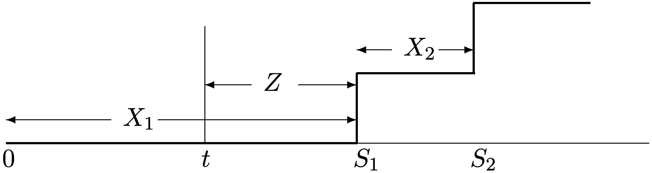
Let \(Z\) be the distance from \(t\) until the first arrival after \(t\). We first condition on \(N(t)=0\) (see Figure 2.2). Given \(N(t)=0\), we see that \(X_{1}>t\) and \(Z=X_{1}-t\). Thus,
\(\begin{aligned}
\operatorname{Pr}\{Z>z \mid N(t)=0\} &=\operatorname{Pr}\left\{X_{1}>z+t \mid N(t)=0\right\} \\
&=\operatorname{Pr}\left\{X_{1}>z+t \mid X_{1}>t\right\} &(2.6)\\
&=\operatorname{Pr}\left\{X_{1}>z\right\}=e^{-\lambda z}&(2.7)
\end{aligned}\)
In (2.6), we used the fact that \(\{N(t)=0\}=\left\{X_{1}>t\right\}\), which is clear from Figure 2.1 (and also from (2.3)). In \ref{2.7} we used the memoryless condition in \ref{2.5} and the fact that \(X_{1}\) is exponential.
Next consider the conditions that \(N(t)=n\) (for arbitrary \(n>1\)) and \(S_{n}=\tau\) (for arbitrary \(\tau \leq t\)). The argument here is basically the same as that with \(N(t)=0\), with a few extra details (see Figure 2.3).
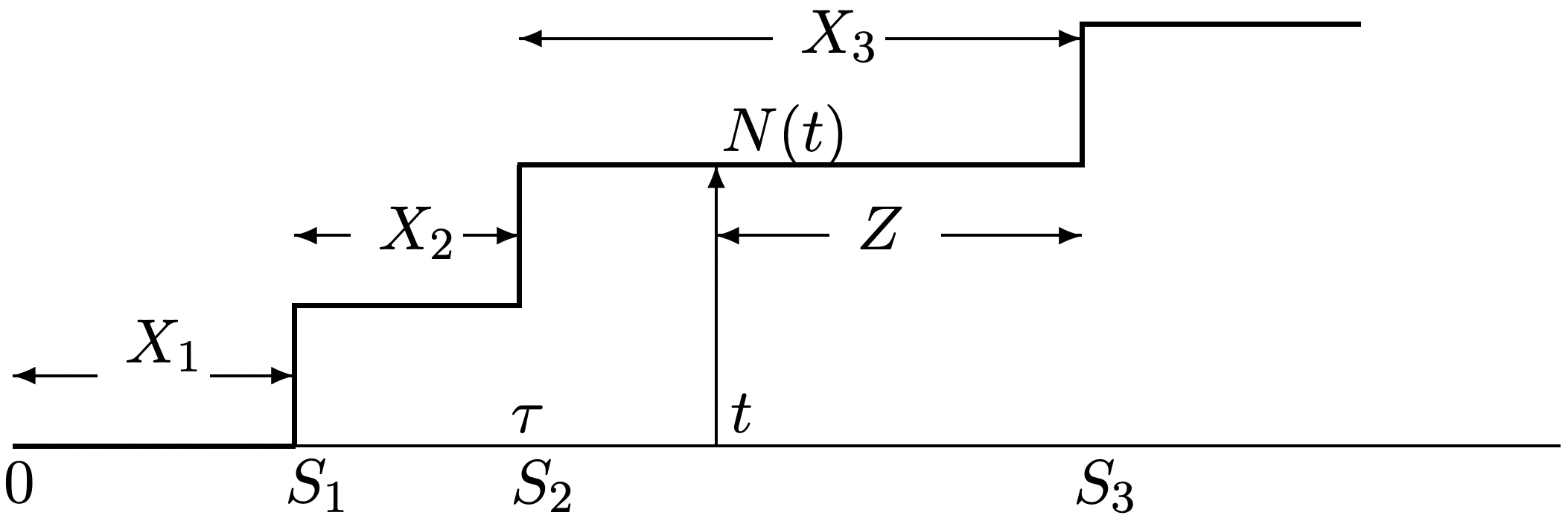
Conditional on \(N(t)=n\) and \(S_{n}=\tau\), the first arrival after \(t\) is the first arrival after the arrival at \(S_{n}\), i.e., \(Z=z\) corresponds to \(X_{n+1}=z+(t-\tau)\).
\(\begin{aligned}
\operatorname{Pr}\left\{Z>z \mid N(t)=n, S_{n}=\tau\right\} &=\operatorname{Pr}\left\{X_{n+1}>z+t-\tau \mid N(t)=n, S_{n}=\tau\right\} &(2.8)\\
&=\operatorname{Pr}\left\{X_{n+1}>z+t-\tau \mid X_{n+1}>t-\tau, S_{n}=\tau\right\} &(2.9)\\
&=\operatorname{Pr}\left\{X_{n+1}>z+t-\tau \mid X_{n+1}>t-\tau\right\} &(2.10)\\
&=\operatorname{Pr}\left\{X_{n+1}>z\right\}=e^{-\lambda z}&(2.11)
\end{aligned}\)
where \ref{2.9} follows because, given \(S_{n}=\tau \leq t\), we have \(\{N(t)=n\}=\left\{X_{n+1}>t-\tau\right\}\) (see Figure 2.3). Eq. \ref{2.10} follows because \(X_{n+1}\) is independent of \(S_{n}\). Eq. \ref{2.11} follows from the memoryless condition in \ref{2.5} and the fact that \(X_{n+1}\) is exponential.
The same argument applies if, in (2.8), we condition not only on \(S_{n}\) but also on \(S_{1}, \ldots, S_{n-1}\). Since this is equivalent to conditioning on \(N(\tau)\) for all \(\tau\) in \((0, t]\), we have
\[\operatorname{Pr}\{Z>z \mid\{N(\tau), 0<\tau \leq t\}\}=\exp (-\lambda z)\label{2.12} \]
Next consider subsequent interarrival intervals after a given time \(t\). For \(m \geq 2\), let \(Z_{m}\) be the interarrival interval from the \(m-1 \mathrm{st}\) arrival epoch after \(t\) to the \(m\)th arrival epoch after \(t\). Let \(Z\) in \ref{2.12} be denoted as \(Z_{1}\) here. Given \(N(t)=n\) and \(S_{n}=\tau\), we see that \(Z_{m}=X_{m+n}\) for \(m \geq 2\), and therefore \(Z_{1}\), \(Z_{2}\), . . ., are IID exponentially distributed rv’s, conditional on \(N(t)=n\) and \(S_{n}=\tau\) (see Exercise 2.8). Since this is independent of \(N(t)\) and \(S_{n}\), we see that \(Z_{1}, Z_{2}, \ldots\) are unconditionally IID and also independent of \(N(t)\) and \(S_{n}\). It should also be clear that \(Z_{1}, Z_{2}, \ldots\) are independent of \(\{N(\tau) ; 0<\tau \leq t\}\).
The above argument shows that the portion of a Poisson process starting at an arbitrary time \(t>0\) is a probabilistic replica of the process starting at 0; that is, the time until the first arrival after \(t\) is an exponentially distributed rv with parameter \(\lambda\), and all subsequent arrivals are independent of this first arrival and of each other and all have the same exponential distribution.
Definition 2.2.4.
A counting process \(\{N(t) ; t>0\}\) has the stationary increment property if for every \(t^{\prime}>t>0, N\left(t^{\prime}\right)-N(t)\) has the same distribution function as \(N\left(t^{\prime}-t\right)\).
Let us define \(\tilde{N}\left(t, t^{\prime}\right)=N\left(t^{\prime}\right)-N(t)\) as the number of arrivals in the interval \(\left(t, t^{\prime}\right]\) for any given \(t^{\prime} \geq t\). We have just shown that for a Poisson process, the rv \(\widetilde{N}\left(t, t^{\prime}\right)\) has the same distribution as \(N\left(t^{\prime}-t\right)\), which means that a Poisson process has the stationary increment property. Thus, the distribution of the number of arrivals in an interval depends on the size e of the interval but not on its starting point.
Definition 2.2.5.
A counting process \(\{N(t) ; t>0\}\) has the independent increment property if, for every integer \(k>0\), and every k-tuple of times \(0<t_{1}<t_{2}<\cdots<t_{k}\), the k-tuple of rv’s \(N\left(t_{1}\right)\), \(\widetilde{N}\left(t_{1}, t_{2}\right)\), . . . , \(\tilde{N}\left(t_{k-1}, t_{k}\right)\) of rv’s are statistically independent.
For the Poisson process, Theorem 2.2.1 says that for any \(t\), the time \(Z_{1}\) until the next arrival after \(t\) is independent of \(N(\tau)\) for all \(\tau \leq t\). Letting \(t_{1}<t_{2}<\cdots t_{k-1}< t\), this means that \(Z_{1}\) is independent of \(N\left(t_{1}\right), \tilde{N}\left(t_{1}, t_{2}\right), \ldots, \tilde{N}\left(t_{k-1}, t\right)\). We have also seen that the subsequent interarrival times after \(Z_{1}\), and thus \(\widetilde{N}\left(t, t^{\prime}\right)\) are independent of \(N\left(t_{1}\right), \widetilde{N}\left(t_{1}, t_{2}\right), \ldots, \widetilde{N}\left(t_{k-1}, t\right)\). Renaming \(t\) as \(t_{k}\) and \(t^{\prime}\) as \(t_{k+1}\), we see that \(\tilde{N}\left(t_{k}, t_{k+1}\right)\) is independent of \(N\left(t_{1}\right), \widetilde{N}\left(t_{1}, t_{2}\right), \ldots, \widetilde{N}\left(t_{k-1}, t_{k}\right)\). Since this is true e for all \(k\), the Poisson process has the independent increment property. In summary, we have proved the e following:
Theorem 2.2.2.
Poisson processes have both the stationary increment and independent increment properties.
Note that if we look only at integer times, then the Bernoulli process also has the stationary and independent increment properties.
Probability density of Sn and S1, . . . Sn
Recall from \ref{2.1} that, for a Poisson process, \(S_{n}\) is the sum of \(n\) IID rv’s, each with the density function \(\mathrm{f}_{X}(x)=\lambda \exp (-\lambda x)\), \(x \geq 0\). Also recall that the density of the sum of two independent rv’s can be found by convolving their densities, and thus the density of \(S_{2}\) can be found by convolving \(\mathrm{f}_{X}(x)\) with itself, \(S_{3}\) by convolving the density of \(S_{2}\) with \(f_{X}(x)\), and so forth. The result, for \(t \geq 0\), is called the Erlang density,5
\[\mathrm{f}_{S_{n}}(t)=\frac{\lambda^{n} t^{n-1} \exp (-\lambda t)}{(n-1) !}\label{2.13} \]
We can understand this density (and other related matters) much better by reviewing the above mechanical derivation more carefully. The joint density for two continuous independent rv’s \(X_{1}\) and \(X_{2}\) is given by \(\mathrm{f}_{X_{1} X_{2}}\left(x_{1}, x_{2}\right)=\mathrm{f}_{X_{1}}\left(x_{1}\right) \mathrm{f}_{X_{2}}\left(x_{2}\right)\). Letting \(S_{2}=X_{1}+X_{2}\) and substituting \(S_{2}-X_{1}\) for \(X_{2}\), we get the following joint density for \(X_{1}\) and the sum \(S_{2}\),
\(\mathrm{f}_{X_{1} S_{2}}\left(x_{1}, s_{2}\right)=\mathrm{f}_{X_{1}}\left(x_{1}\right) \mathrm{f}_{X_{2}}\left(s_{2}-x_{1}\right)\)
The marginal density for \(S_{2}\) then results from integrating \(x_{1}\) out from the joint density, and this, of course, is the familiar convolution integration. For IID exponential rv’s \(X_{1}, X_{2}\), the joint density of \(X_{1}, S_{2}\) takes the following interesting form:
\[\mathrm{f}_{X_{1} S_{2}}\left(x_{1} s_{2}\right)=\lambda^{2} \exp \left(-\lambda x_{1}\right) \exp \left(-\lambda\left(s_{2}-x_{1}\right)\right)=\lambda^{2} \exp \left(-\lambda s_{2}\right) \quad\text { for } 0 \leq x_{1} \leq s_{2}\label{2.14} \]
This says that the joint density does not contain \(x_{1}\), except for the constraint \(0 \leq x_{1} \leq s_{2}\). Thus, for fixed \(s_{2}\), the joint density, and thus the conditional density of \(X_{1}\) given \(S_{2}=s_{2}\) is uniform over \(0 \leq x_{1} \leq s_{2}\). The integration over \(x_{1}\) in the convolution equation is then simply multiplication by the interval size \(s_{2}\), yielding the marginal distribution \(\mathrm{f}_{S_{2}}\left(s_{2}\right)=\lambda^2s_2\mathrm{exp}(-\lambda s_2)\), in agreement with \ref{2.13} for \(n = 2\).
This same curious behavior exhibits itself for the sum of an arbitrary number \(n\) of IID exponential rv’s. That is, \(\mathrm{f}_{X_{1} \cdots X_{n}}\left(x_{1}, \ldots, x_{n}\right)=\lambda^{n} \exp \left(-\lambda x_{1}-\lambda x_{2}-\cdots-\lambda x_{n}\right)\). Letting \(S_{n}=X_{1}+\cdots+X_{n}\) and substituting \(S_{n}-X_{1}-\cdots-X_{n-1}\) for \(X_{n}\), this becomes
\(\mathrm{f}_{X_{1} \cdots X_{n-1} S_{n}}\left(x_{1}, \ldots, x_{n-1}, s_{n}\right)=\lambda^{n} \exp \left(-\lambda s_{n}\right)\)
since each \(x_{i}\) cancels out above. This equation is valid over the region where each \(x_{i} \geq 0\) and \(s_{n}-x_{1}-\cdots-x_{n-1} \geq 0\). The density is 0 elsewhere.
The constraint region becomes more clear here if we replace the interarrival intervals \(X_{1}, \ldots, X_{n-1}\) with the arrival epochs \(S_{1}, \ldots, S_{n-1}\) where \(S_{1}=X_{1}\) and \(S_{i}=X_{i}+S_{i-1}\) for \(2 \leq i \leq n-1\). The joint density then becomes6
\[\mathrm{f}_{S_{1} \cdots S_{n}}\left(s_{1}, \ldots, s_{n}\right)=\lambda^{n} \exp \left(-\lambda s_{n}\right) \quad \text { for } 0 \leq s_{1} \leq s_{2} \cdots \leq s_{n}\label{2.15} \]
The interpretation here is the same as with \(S_{2}\). The joint density does not contain any arrival time other than \(\boldsymbol{s}_{n}\), except for the ordering constraint \(0 \leq s_{1} \leq s_{2} \leq \cdots \leq s_{n}\), and thus this joint density is constant over all choices of arrival times satisfying the ordering constraint. Mechanically integrating this over \(s_{1}\), then \(s_{2}\), etc. we get the Erlang formula (2.13). The Erlang density then is the joint density in \ref{2.15} times the volume \(s_{n}^{n-1} /(n-1)!\) of the region of \(s_{1}, \ldots, s_{n-1}\) satisfing \(0<s_{1}<\cdots<s_{n}\). This will be discussed further later.
Note that (2.15), for all \(n\) specifies the joint distribution for all arrival times, and thus fully specifes a Poisson process. An alternate definition for the Poisson process is then any process whose joint arrival time distribution satisifes (2.15). This is not customarily used to define the Poisson process, whereas two alternate definitions given subsequently often are used as a starting definition.
for N(t)
The Poisson counting process, \(\{N(t) ; t>0\}\) consists of a nonnegative integer rv \(N(t)\) for each \(t>0\). In this section, we show that the PMF for this rv is the well-known Poisson PMF, as stated in the following theorem. We give two proofs for the theorem, each providing its own type of understanding and each showing the close relationship between \(\{N(t)=n\}\) and \(\left\{S_{n}=t\right\}\).
Theorem 2.2.3.
For a Poisson process of rate \(\lambda\), and for any \(t>0\), the PMF for \(N(t)\) (i.e., the number of arrivals in \((0, t]\)) is given by the Poisson PMF,
\[\mathbf{p}_{N(t)}(n)=\frac{(\lambda t)^{n} \exp (-\lambda t)}{n !}\label{2.16} \]
Proof 1: This proof, for given \(n\) and \(t\), is based on two ways of calculating \(\operatorname{Pr}\left\{t<S_{n+1} \leq t+\delta\right\}\) for some vanishingly small \(\delta\). The first way is based on the already known density of \(S_{n+1}\) and gives
\(\operatorname{Pr}\left\{t<S_{n+1} \leq t+\delta\right\}=\int_{t}^{\}{t+\delta}} \mathrm{f}_{S_{n}}(\tau) d \tau=\mathrm{f}_{S_{n}}(t)(\delta+o(\delta))\)
The term \(o(\delta)\) is used to describe a function of \(\delta\) that goes to 0 faster than \(\delta\) as \(\delta \rightarrow 0\). More precisely, a function \(g(\delta)\) is said to be of order \(o(\delta)\) if \(\lim _{\delta \rightarrow 0} \frac{g(\delta)}{\delta}=0\). Thus \(\operatorname{Pr}\left\{t<S_{n} \leq t+\delta\right\}=\mathrm{f}_{S_{n}}(t)(\delta+o(\delta))\) is simply a consequence of the fact that \(S_{n}\) has a continuous probability density in the interval \([t, t+\delta]\).
The second way to calculate \(\operatorname{Pr}\left\{t<S_{n+1} \leq t+\delta\right\}\) is to first observe that the probability of more than 1 arrival in \((t, t+\delta])\) is \(o(\delta)\). Ignoring this possibility, \(\left\{t<S_{n+1} \leq t+\delta\right\}\) occurs if exactly \(n\) arrivals are in the interval \((0, t]\) and one arrival occurs in \((t, t+\delta]\). Because of the independent increment property, this is an event of probability \(\mathbf{p}_{N(t)}(n)(\lambda \delta+o(\delta))\).
Thus
\(\mathrm{p}_{N(t)}(n)(\lambda \delta+o(\delta))+o(\delta)=\mathrm{f}_{S_{n+1}}(t)(\delta+o(\delta))\)
Dividing by \(\delta\) and taking the limit \(\delta \rightarrow 0\), we get
\(\lambda \mathbf{p}_{N(t)}(n)=\mathbf{f}_{S_{n+1}}(t)\)
Using the density for \(\mathrm{f}_{S_{n}}\) in (2.13), we get (2.16).
Proof 2: The approach here is to use the fundamental relation that \(\{N(t) \geq n\}=\left\{S_{n} \leq t\right\}\). Taking the probabilities of these events,
\(\begin{aligned}
&\sum_{i=n}^{\infty} \mathrm{p}_{N(t)}(i)=\int_{0}^{\}t} \mathrm{f}_{S_{n}}(\tau) d \tau
&\text { for all } n \geq 1 \text { and } t>0
\end{aligned}\)
The term on the right above is the distribution function of \(S_{n}\) and the term on the left is the complementary distribution function of \(N(t)\). The complementary distribution function and the PMF of \(N(t)\) uniquely specify each other, so the theorem is equivalent to showing that
\[\sum_{i=n}^{\infty} \frac{(\lambda t)^{i} \exp (-\lambda t)}{i !}=\int_{0}^{\}t} \mathrm{f}_{S_{n}}(\tau) d \tau\label{2.17} \]
If we take the derivative with respect to t of each side of (2.17), we find that almost magically each term except the first on the left cancels out, leaving us with
\(\frac{\lambda^{n} t^{n-1} \exp (-\lambda t)}{(n-1) !}=\mathrm{f}_{S_{n}}(t)\)
Thus the derivative with respect to \(t\) of each side of \ref{2.17} is equal to the derivative of the other for all \(n \geq 1\) and \(t>0\). The two sides of \ref{2.17} are also equal in the limit \(t \rightarrow 0\), so it follows that \ref{2.17} is satisfied everywhere, completing the proof.
Alternate definitions of Poisson processes
A Poisson counting process \(\{N(t) ; t>0\}\) is a counting process that satisfies \ref{2.16} (i.e., has the Poisson PMF) and has the independent and stationary increment properties.
We have seen that the properties in Definition 2 are satisfied starting with Definition 1 (using IID exponential interarrival times), so Definition 1 implies Definition 2. Exercise 2.4 shows that IID exponential interarrival times are implied by Definition 2, so the two definitions are equivalent.
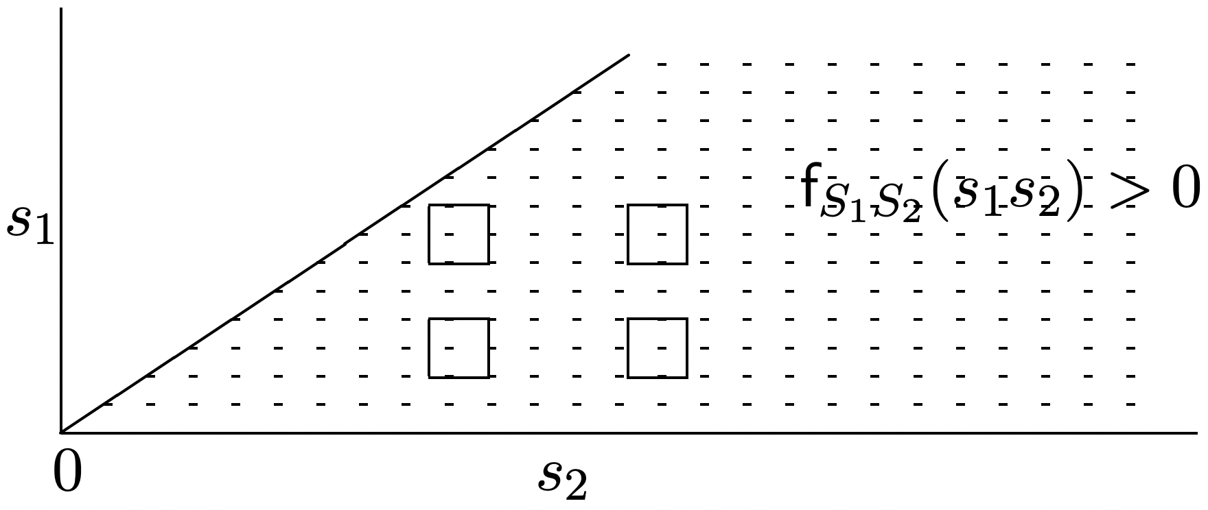
It may be somewhat surprising at first to realize that a counting process that has the Poisson PMF at each t is not necessarily a Poisson process, and that the independent and stationary increment properties are also necessary. One way to see this is to recall that the Poisson PMF for all t in a counting process is equivalent to the Erlang density for the successive arrival epochs. Specifying the probability density for \(S_{1}\), \(S_{2}\), . . . , as Erlang specifies the marginal densities of \(S_{1}\), \(S_{2}\), . . , but need not specify the joint densities of these rv’s. Figure 2.4 illustrates this in terms of the joint density of \(S_{1}\), \(S_{2}\), given as
\(\mathrm{f}_{S_{1} S_{2}}\left(s_{1} s_{2}\right)=\lambda^{2} \exp \left(-\lambda s_{2}\right) \quad \text { for } 0 \leq s_{1} \leq s_{2}\)
and 0 elsewhere. The figure illustrates how the joint density can be changed without changing the marginals.
There is a similar effect with the Bernoulli process in that a discrete counting process for which the number of arrivals from 0 to \(t\), for each integer \(t\), is a binomial rv, but the process is not Bernoulli. This is explored in Exercise 2.5.
The next definition of a Poisson process is based on its incremental properties. Consider the number of arrivals in some very small interval \((t, t+\delta]\). Since \(\tilde{N}(t, t+\delta)\) has the same distribution as \(N(\delta)\), we can use \ref{2.16} to get
\[\begin{aligned}
&\operatorname{Pr}\{\tilde{N}(t, t+\delta)=0\}^\}=e^{-\lambda \delta} \approx 1-\lambda \delta+o(\delta) \\
&\operatorname{Pr}\{\tilde{N}(t, t+\delta)=1\}^\}=\lambda \delta e^{-\lambda \delta} \approx \lambda \delta+o(\delta) \\
&\operatorname{Pr}\{\tilde{N}(t, t+\delta) \geq 2\}^\} \approx o(\delta)
\end{aligned}\label{2.18} \]
A Poisson counting process is a counting process that satisfies \ref{2.18} and has the stationary and independent increment properties.
We have seen that Definition 1 implies Definition 3. The essence of the argument the other way is that for any interarrival interval \(X\), \(\mathrm{F}_{X}(x+\delta)-\mathrm{F}_{X}(x)\) is the probability of an arrival in an appropriate infinitesimal interval of width \(\delta\), which by \ref{2.18} is \(\lambda \delta+o(\delta)\). Turning this into a differential equation (see Exercise 2.7), we get the desired exponential interarrival intervals. Definition 3 has an intuitive appeal, since it is based on the idea of independent arrivals during arbitrary disjoint intervals. It has the disadvantage that one must do a considerable amount of work to be sure that these conditions are mutually consistent, and probably the easiest way is to start with Definition 1 and derive these properties. Showing that there is a unique process that satisfies the conditions of Definition 3 is even harder, but is not necessary at this point, since all we need is the use of these properties. Section 2.2.5 will illustrate better how to use this definition (or more precisely, how to use (2.18)).
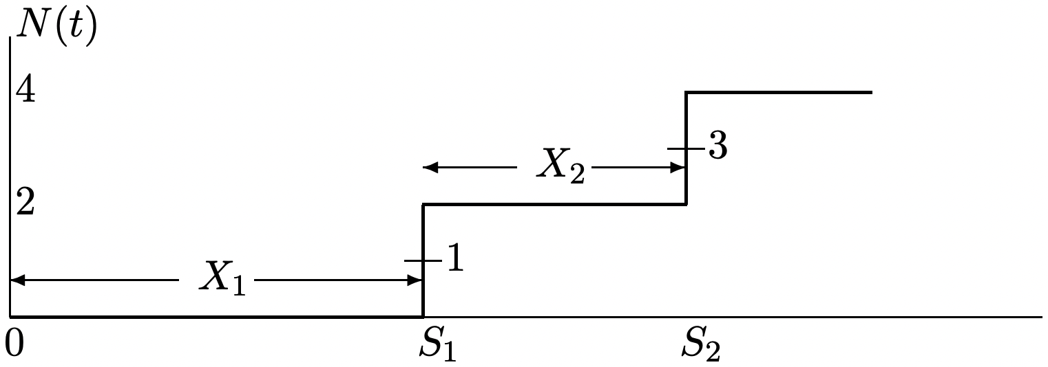
What \ref{2.18} accomplishes in Definition 3, beyond the assumption of independent and stationary increments, is the prevention of bulk arrivals. For example, consider a counting process in which arrivals always occur in pairs, and the intervals between successive pairs are IID and exponentially distributed with parameter \(\lambda\) (see Figure 2.5). For this process, \(\operatorname{Pr}\{\widetilde{N}(t, t+\delta)=1\}^\}=0, \text { and } \operatorname{Pr}\{\widetilde{N}(t, t+\delta)=2\}^\}=\lambda \delta+o(\delta)\), thus violating (2.18). This process has stationary and independent increments, however, since the process formed by viewing a pair of arrivals as a single incident is a Poisson process.
Poisson process as a limit of shrinking Bernoulli processes
The intuition of Definition 3 can be achieved in a less abstract way by starting with the Bernoulli process, which has the properties of Definition 3 in a discrete-time sense. We then go to an appropriate limit of a sequence of these processes, and find that this sequence of Bernoulli processes converges in some sense to the Poisson process.
Recall that a Bernoulli process is an IID sequence, \(Y_{1}, Y_{2}, \ldots\), of binary random variables for which \(\mathrm{p}_{Y}(1)=p\) and \(\mathrm{p}_{Y}(0)=1-p\). We can visualize \(Y_{i}=1\) as an arrival at time \(i\) and \(Y_{i}=0\) as no arrival, but we can also ‘shrink’ the time scale of the process so that for some integer \(j>0\), \(Y_{i}\) is an arrival or no arrival at time \(i 2^{-j}\). We consider a sequence indexed
by \(j\) of such shrinking Bernoulli processes, and in order to keep the arrival rate constant, we let \(p=\lambda 2^{-j}\) for the \(j \text { th }\) process. Thus for each unit increase in \(j\), the Bernoulli process shrinks by replacing each slot with two slots, each with half the previous arrival probability. The expected number of arrivals per unit time is then , matching the Poisson process that we are approximating.
If we look at this \(j \text { th }\) process relative to Definition 3 of a Poisson process, we see that for these regularly spaced increments of size \(\delta=2^{-j}\), the probability of one arrival in an increment is \(\lambda \delta\) and that of no arrival is \(1-\lambda \delta\), and thus \ref{2.18} is satisfied, and in fact the \(o(\delta)\) terms are exactly zero. For arbitrary sized increments, it is clear that disjoint increments have independent arrivals. The increments are not quite stationary, since, for example, an increment of size \(2^{-j-1}\) might contain a time that is a multiple of \(2^{-j}\) or might not, depending on its placement. However, for any fixed increment of size \(\delta\), the number of multiples of \(2^{-j}\) (i.e., the number of possible arrival points) is either \(\left\lfloor\delta 2^{j}\right\rfloor\) or \(1+\left\lfloor\delta 2^{j}\right\rfloor\). Thus in the limit \(j \rightarrow \infty\), the increments are both stationary and independent.
For each \(j\), the \(j \text { th }\) Bernoulli process has an associated Bernoulli counting process \(N_j(t)=\sum_{i=1}^{\left\lfloor t 2^{j}\right\rfloor} Y_{i}\). This is the number of arrivals up to time \(t\) and is a discrete rv with the binomial i=1 PMF. That is, \(\mathbf{p}_{N_{j}(t)}(n)=\left(\begin{array}{c}
\left\lfloor t 2^{j}\right\rfloor \\ n \end{array}\right) p^{n}(1-p)^{\left\lfloor t 2^{j}\right\rfloor-n}\) where \(p=\lambda 2^{-j}\). We now show that this PMF approaches the Poisson PMF as \(j\) increases.7
Theorem 2.2.4.
Consider the sequence of shrinking Bernoulli processes with arrival probability \(\lambda 2^{-j}\) and time-slot size \(2^{-j}\). Then for every fixed time \(t>0\) and fixed number of arrivals \(n\), the counting PMF \(\mathbf{p}_{N_{j}(t)}(n)\) approaches the Poisson PMF (of the same \(\lambda\)) with increasing \(j\), i.e.,
\[\lim _{j \rightarrow \infty} \mathrm{p}_{N_{j}(t)}(n)=\mathrm{p}_{N(t)}(n)\label{2.19} \]
Proof: We first rewrite the binomial PMF, for \(\left\lfloor t 2^{j}\right\rfloor\) variables with \(p=\lambda 2^{-j}\) as
\[\begin{aligned}
\lim _{j \rightarrow \infty} p_{N_{j}(t)}(n) &=\lim _{j \rightarrow \infty}\left(\begin{array}{c}
\left\lfloor t 2^{j}\right\rfloor \\ n
\end{array}\right)\left(\frac{\} \lambda 2^{-j}}{1-\lambda 2^{-j}}\right)^{\}n} \exp \left[\left\lfloor t 2^{j}\right\rfloor\left(\ln \left(1-\lambda 2^{-j}\right)\right]\right.\\
&=\lim _{j \rightarrow \infty}\left(\begin{array}{c}
\left\lfloor t 2^{j}\right\rfloor \\ n
\end{array}\right)\left(\frac{3 \lambda 2^{-j}}{1-\lambda 2^{-j}}\right)^{\}n} \exp (-\lambda t) &(2.20)\\
&=\lim _{j \rightarrow \infty} \frac{\left\lfloor t 2^{j}\right\rfloor \cdot\left\lfloor t 2^{j}-1\right\rfloor \cdots\left\lfloor t 2^{j}-n+1\right\rfloor}{n !}\left(\frac{\} \lambda 2^{-j}}{1-\lambda 2^{-j}}\right)^{\}n} \exp (-\lambda t) &(2.21)\\
&=\frac{(\lambda t)^{n} \exp (-\lambda t)}{n !} &(2.22)
\end{aligned} \nonumber \]
We used \(\ln \left(1-\lambda 2^{-j}\right)=-\lambda 2^{-j}+o\left(2^{-j}\right)\) in \ref{2.20} and expanded the combinatorial term in (2.21). In (2.22), we recognized that \(\lim _{j \rightarrow \infty}\left\lfloor t 2^{j}-i\right\rfloor\left(\frac{\} \lambda 2^{-j}}{1-\lambda 2^{-j}}\right)^{\}}=\lambda t \text { for } 0 \leq i \leq n-1\).
Since the binomial PMF (scaled as above) has the Poisson PMF as a limit for each \(n\), the distribution function of \(N_{j}(t)\) also converges to the Poisson distribution function for each \(t\). In other words, for each \(t>0\), the counting random variables \(N_{j}(t)\) of the Bernoulli processes converge in distribution to \(N(t)\) of the Poisson process.
This does not say that the Bernoulli counting processes converge to the Poisson counting process in any meaningful sense, since the joint distributions are also of concern. The following corollary treats this.
Corollary 2.2.1.
For any finite integer \(k>0\), let \(0<t_{1}<t_{2}<\cdots<t_{k}\) be any set of time instants. Then the joint distribution function of \(N_{j}\left(t_{1}\right), N_{j}\left(t_{2}\right), \ldots N_{j}\left(t_{k}\right)\) approaches the joint distribution function of \(N\left(t_{1}\right), N\left(t_{2}\right), \ldots N\left(t_{k}\right)\) as \(j \rightarrow \infty\).
Proof: It is sucient to show that the joint PMF’s converge. We can rewrite the joint PMF for each Bernoulli process as
\[\begin{aligned}
\mathrm{p}_{N_{j}\left(t_{1}\right), \ldots, N_{j}\left(t_{k}\right)}\left(n_{1}, \ldots, n_{k}\right) &=\mathrm{p}_{N_{j}\left(t_{1}\right), \tilde{N}_{j}\left(t_{1}, t_{2}\right), \ldots, \tilde{N}_{j}\left(t_{k-1}, t_{k}\right)}\left(n_{1}, n_{2}-n_{1}, \ldots, n_{k}-n_{k-1}\right) \\
&=\mathrm{p}_{N_{j}\left(t_{1}\right)}\left(n_{1}\right) \prod_{\ell=2}^{k} \mathrm{p}_{\tilde{N}_{j}\left(t_{\ell}, t_{\ell-1}\right)}\left(n_{\ell}-n_{\ell-1}\right)
\end{aligned}\label{2.23} \]
where we have used the independent increment property for the Bernoulli process. For the Poisson process, we similarly have
\[\mathrm{p}_{N\left(t_{1}\right), \ldots, N\left(t_{k}\right)}\left(n_{1}, \ldots n_{k}\right)=\mathrm{p}_{N\left(t_{1}\right)}\left(n_{1}\right) \prod_{\ell=2}^{k} \mathrm{p}_{\tilde{N}\left(t_{\ell}, t_{\ell-1}\right)}\left(n_{\ell}-n_{\ell-1}\right)\label{2.24} \]
Taking the limit of \ref{2.23} as \(j \rightarrow \infty\), we recognize from Theorem 2.2.4 that each term of \ref{2.23} goes to the corresponding term in (2.24). For the \(\tilde{N}\) rv’s , this requires a trivial generalization in Theorem 2.2.4 to deal with the arbitrary starting time.
We conclude from this that the sequence of Bernoulli processes above converges to the Poisson process in the sense of the corollary. Recall from Section 1.5.5 that there are a number of ways in which a sequence of rv’s can converge. As one might imagine, there are many more ways in which a sequence of stochastic processes can converge, and the corollary simply establishes one of these. We have neither the mathematical tools nor the need to delve more deeply into these convergence issues.
Both the Poisson process and the Bernoulli process are so easy to analyze that the convergence of shrinking Bernoulli processes to Poisson is rarely the easiest way to establish properties about either. On the other hand, this convergence is a powerful aid to the intuition in understanding each process. In other words, the relation between Bernoulli and Poisson is very useful in suggesting new ways of looking at problems, but is usually not the best way to analyze those problems.
Reference
4With this density, \(\operatorname{Pr}\left\{X_{i}>0\right\}=1\), so that we can regard \(X_{i}\) as a positive random variable. Since events of probability zero can be ignored, the density \(\lambda \exp (-\lambda x)\) for \(x \geq 0\) and zero for \(x<0\) is effectively the same as the density \(\lambda \exp (-\lambda x)\) for \(x>0\) and zero for \(x \leq 0\).
5Another (somewhat rarely used) name for the Erlang density is the gamma density.
6The random vector \(\boldsymbol{S}=\left(S_{1}, \ldots, S_{n}\right)\) is then related to the interarrival intervals \(\boldsymbol{X}=\left(X_{1}, \ldots, X_{n}\right)\) by a linear transformation, say \(\boldsymbol{S}=\mathbf{A} \boldsymbol{X}\) where A is an upper triangular matrix with ones on the main diagonal and on all elements above the main diagonal. In general, the joint density of a non-singular linear transformation \(A X\) at \(\boldsymbol{X}=\boldsymbol{x}\) is \(\mathrm{f}_{\boldsymbol{X}}(\boldsymbol{x}) /|\operatorname{det} \mathrm{A}|\). This is because the transformation A carries an incremental cube, \(\delta\) on each side, into a parallelepiped of volume \(\delta^{n}|\operatorname{det} \mathrm{A}|\). Since, for the case here, A is upper triangular with 1’s on the diagonal, det A=1.
7This limiting result for the binomial distribution is very different from the asymptotic results in Chapter 1 for the binomial. Here the parameter \(p\) of the binomial is shrinking with increasing \(j\), whereas there, \(p\) is constant while the number of variables is increasing.