2.3: Combining and Splitting Poisson Processes

Suppose that ; : \(t>0\}\) and \(\left\{N_{2}(t) ; t>0\right\}\) are independent Poisson counting processes⁸ of rates \(\lambda_{1}\) and \(\lambda_{2}\) respectively. We want to look at the sum process where \(N(t)=N_{1}(t)+N_{2}(t)\) for all \(t \geq 0\). In other words, \(\{N(t) ; t>0\}\) is the process consisting of all arrivals to both process 1 and process 2. We shall show that \(\{N(t) ; t>0\}\) is a Poisson counting process of rate \(\lambda=\lambda_{1}+\lambda_{2}\). We show this in three different ways, first using Definition 3 of a Poisson process (since that is most natural for this problem), then using Definition 2, and finally Definition 1. We then draw some conclusions about the way in which each approach is helpful. Since \(\left\{N_{1}(t) ; t>0\right\}\) and \(\left\{N_{2}(t) ; t>0\right\}\) are independent and each possess the stationary and independent increment properties, it follows from the definitions that \(\{N(t) ; t>0\}\) also possesses the stationary and independent increment properties. Using the approximations in \ref{2.18} for the individual processes, we see that

\(\begin{aligned}
\operatorname{Pr}\{\tilde{N}(t, t+\delta)=0\}\} &=\operatorname{Pr}\left\{\tilde{N}_{1}(t, t+\delta)=0\right\} \operatorname{Pr}\left\{\tilde{N}_{2}(t, t+\delta)=0\right\} \\
&=\left(1-\lambda_{1} \delta\right)\left(1-\lambda_{2} \delta\right) \approx 1-\lambda \delta
\end{aligned}\)

where \(\lambda_{1} \lambda_{2} \delta^{2}\) has been dropped. In the same way, \(\operatorname{Pr}\{\tilde{N}(t, t+\delta)=1\}^\}\) is approximated by \(\lambda \delta\) and \(\operatorname{Pr}\{\widetilde{N}(t, t+\delta) \geq 2\}^\}\) is approximated by 0, both with errors proportional to \(\delta^{2}\). It follows that \(\{N(t) ; t>0\}\) is a Poisson process.

In the second approach, we have \(N(t)=N_{1}(t)+N_{2}(t)\). Since \(N(t)\), for any given \(t\), is the sum of two independent Poisson rv’s , it is also a Poisson rv with mean \(\lambda t=\lambda_{1} t+\lambda_{2} t\). If the reader is not aware that the sum of two independent Poisson rv’s is Poisson, it can be derived by discrete convolution of the two PMF’s (see Exercise 1.19). More elegantly, one can observe that we have already implicitly shown this fact. That is, if we break an interval \(I\) into disjoint subintervals, \(I_{1}\) and \(I_{2}\), then the number of arrivals in \(I\) (which is Poisson) is the sum of the number of arrivals in \(I_{1}\) and in \(I_{2}\) (which are independent Poisson).

Finally, since \(N(t)\) is Poisson for each \(t\), and since the stationary and independent increment properties are satisfied, \(\{N(t) ; t>0\}\) is a Poisson process.

In the third approach, \(X_{1}\), the first interarrival interval for the sum process, is the minimum of \(X_{11}\), the first interarrival interval for the first process, and \(X_{21}\), the first interarrival interval for the second process. Thus \(X_{1}>t\), if and only if both \(X_{11}\) and \(X_{21}\) exceed \(t\), so

\(\operatorname{Pr}\left\{X_{1}>t\right\}=\operatorname{Pr}\left\{X_{11}>t\right\} \operatorname{Pr}\left\{X_{21}>t\right\}=\exp \left(-\lambda_{1} t-\lambda_{2} t\right)=\exp (-\lambda t)\)

Using the memoryless property, each subsequent interarrival interval can be analyzed in the same way.

The first approach above was the most intuitive for this problem, but it required constant care about the order of magnitude of the terms being neglected. The second approach was the simplest analytically (after recognizing that sums of independent Poisson rv’s are Poisson), and required no approximations. The third approach was very simple in retrospect, but not very natural for this problem. If we add many independent Poisson processes together, it is clear, by adding them one at a time, that the sum process is again Poisson. What is more interesting is that when many independent counting processes (not necessarily Poisson) are added together, the sum process often tends to be approximately Poisson if the individual processes have small rates compared to the sum. To obtain some crude intuition about why this might be expected, note that the interarrival intervals for each process (assuming no bulk arrivals) will tend to be large relative to the mean interarrival interval for the sum process. Thus arrivals that are close together in time will typically come from different processes. The number of arrivals in an interval large relative to the combined mean interarrival interval, but small relative to the individual interarrival intervals, will be the sum of the number of arrivals from the different processes; each of these is 0 with large probability and 1 with small probability, so the sum will be approximately Poisson.

Subdividing a Poisson process

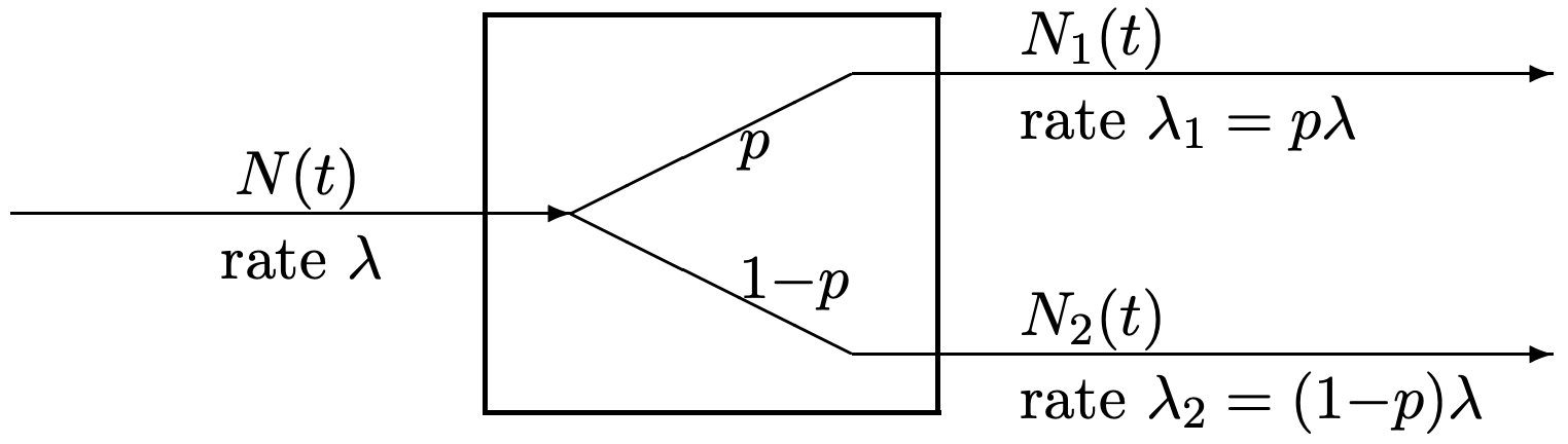
Next we look at how to break \(\{N(t) ; t>0\}\), a Poisson counting process of rate \(\lambda\), into two processes, \(\left\{N_{1}(t) ; t>0\right\}\) and \(\left\{N_{2}(t) ; t>0\right\}\). Suppose that each arrival in \(\{N(t) ; t>0\}\) is sent to the first process with probability \(p\) and to the second process with probability \(1-p\) (see Figure 2.6). Each arrival is switched independently of each other arrival and independently of the arrival epochs. It may be helpful to visualize this as the combination of two independent processes. The first is the Poisson process of rate \(\lambda\) and the second is a Bernoulli process \(\left.X_{n} ; n \geq 1\right\}\) where \(\mathrm{p}_{X_{n}}(1)=p\) and \(\mathrm{p}_{X_{n}}(2)=1-p\). The \(n\)th arrival of the Poisson process is then labeled as a type 1 arrival if \(X_{n}=1\) and as a type 2 arrival with probability \(1-p\).

We shall show that the resulting processes are each Poisson, with rates \(\lambda_{1}=\lambda p\) and \(\lambda_{2}=\lambda(1-p)\) respectively, and that furthermore the two processes are independent. Note that, conditional on the original process, the two new processes are not independent; in fact one completely determines the other. Thus this independence might be a little surprising.

First consider a small increment \((t, t+\delta]\). The original process has an arrival in this incremental interval with probability \(\lambda \delta\) (ignoring \(\delta^{2}\) terms as usual), and thus process 1

Figure 2.6: Each arrival is independently sent to process 1 with probability \(p\) and to process 2 otherwise.

has an arrival with probability p and process 2 with probability \(\lambda \delta(1-p)\). Because of the independent increment property of the original process and the independence of the division of each arrival between the two processes, the new processes each have the independent increment property, and from above have the stationary increment property. Thus each process is Poisson. Note now that we cannot verify that the two processes are independent from this small increment model. We would have to show that the number of arrivals for process 1 and 2 are independent over \((t, t+\delta]\). Unfortunately, leaving out the terms of order \(\delta^{2}\), there is at most one arrival to the original process and no possibility of an arrival to each new process in \((t, t+\delta]\). If it is impossible for both processes to have an arrival in the same interval, they cannot be independent. It is possible, of course, for each process to have an arrival in the same interval, but this is a term of order \(\delta^{2}\). Thus, without paying attention to the terms of order \(\delta^{2}\), it is impossible to demonstrate that the processes are independent.

To demonstrate that process 1 and 2 are independent, we first calculate the joint PMF for \(N_{1}(t)\), \(N_{2}(t)\) for arbitrary \(t\). Conditioning on a given number of arrivals \(N(t)\) for the original process, we have

\[\operatorname{Pr}\left\{N_{1}(t)=m, N_{2}(t)=k \mid N(t)=m+k\right\}=\frac{(m+k) !}{m ! k !} p^{m}(1-p)^{k}\label{2.25} \]

Equation \ref{2.25} is simply the binomial distribution, since, given \(m+k\) arrivals to the original process, each independently goes to process 1 with probability \(p\). Since the event \(\left\{N_{1}(t)=m, N_{2}(t)=k\right\}\) is a subset of the conditioning event above,

\(\operatorname{Pr}\left\{N_{1}(t)=m, N_{2}(t)=k \mid N(t)=m+k\right\}=\frac{\operatorname{Pr}\left\{N_{1}(t)=m, N_{2}(t)=k\right\}}{\operatorname{Pr}\{N(t)=m+k\}}\)

Combining this with (2.25), we have

\[\operatorname{Pr}\left\{N_{1}(t)=m, N_{2}(t)=k\right\}=\frac{(m+k !)}{m ! k !} p^{m}(1-p)^{k} \frac{(\lambda t)^{m+k} e^{-\lambda t}}{(m+k) !}\label{2.26} \]

Rearranging terms, we get

\[\operatorname{Pr}\left\{N_{1}(t)=m, N_{2}(t)=k\right\}=\frac{(p \lambda t)^{m} e^{-\lambda p t}}{m !} \frac{[(1-p) \lambda t]^{k} e^{-\lambda(1-p) t}}{k !}\label{2.27} \]

This shows that \(N_{1}(t)\) and \(N_{2}(t)\) are independent. To show that the processes are independent, we must show that for any \(k>1\) and any set of times \(0 \leq t_{1} \leq t_{2} \leq \cdots \leq t_{k}\), the sets \(\left\{N_{1}\left(t_{i}\right) ; 1 \leq i \leq k\right\}\) and \(\left\{N_{2}\left(t_{j}\right) ; 1 \leq j \leq k\right\}\) are independent of each other. It is equivalent to show that the sets \(\left\{\tilde{N}_{1}\left(t_{i-1}, t_{i}\right) ; 1 \leq i \leq k\right\}\) and \(\left\{\tilde{N}_{2}\left(t_{j-1}, t_{j}\right) ; 1 \leq j \leq k\right\}\) (where \(t_{0}\) is 0) are independent. The argument above shows this independence for \(i=j\), and for \(i \neq j\), the independence follows from the independent increment property of \(\{N(t) ; t>0\}\).

Examples using independent Poisson processes

We have observed that if the arrivals of a Poisson process are split into two new arrival processes, each arrival of the original process independently going into the first of the new processes with some fixed probability \(p\), then the new processes are Poisson processes and are independent. The most useful consequence of this is that any two independent Poisson processes can be viewed as being generated from a single process in this way. Thus, if one process has rate \(\lambda_{1}\) and the other has rate \(\lambda_{2}\), they can be viewed as coming from a process of rate \(\lambda_{1}+\lambda_{2}\). Each arrival to the combined process is then labeled as a first process arrival with probability \(p=\lambda_{1} /\left(\lambda_{1}+\lambda_{2}\right)\) and as a second process arrival with probability \(1-p\).

The above point of view is very useful for finding probabilities such as \(\operatorname{Pr}\left\{S_{1 k}<S_{2 j}\right\}\) where \(S_{1 k}\) is the epoch of the \(k\)th arrival to the first process and \(S_{2 j}\) is the epoch of the \(j\)th arrival to the second process. The problem can be rephrased in terms of a combined process to ask: out of the first \(k+j-1\) arrivals to the combined process, what is the probability that \(k\) or more of them are switched to the first process? (Note that if \(k\) or more of the first \(k+j-1\) go to the first process, at most \(j-1\) go to the second, so the \(k\)th arrival to the first precedes the \(j\)th arrival to the second; similarly if fewer than \(k\) of the first \(k+j-1\) go to the first process, then the \(j\)th arrival to the second process precedes the \(k\)th arrival to the first). Since each of these first \(k+j-1\) arrivals are switched independently with the same probability \(p\), the answer is

\[\operatorname{Pr}\left\{S_{1 k}<S_{2 j}\right\}=\sum_{i=k}^{k+j-1} \frac{(k+j-1) !}{i !(k+j-1-i) !} p^{i}(1-p)^{k+j-1-i}\label{2.28} \]

Example 2.3.1

[The M/M/1 queue] Queueing theorists use a standard notation of characters separated by slashes to describe common types of queueing systems. The first character describes the arrival process to the queue. \(M\) stands for memoryless and means a Poisson arrival process; \(D\) stands for deterministic and means that the interarrival interval is fixed and non-random; \(G\) stands for general interarrival distribution. We assume that the interarrival intervals are IID (thus making the arrival process a renewal process), but many authors use \(\text { GI }\) to explicitly indicate IID interarrivals. The second character describes the service process. The same letters are used, with M indicating an exponential service time distribution. The third character gives the number of servers. It is assumed, when this notation is used, that the service times are IID, independent of the arrival times, and independent of which server is used.

Solution

Consider an M/M/1 queue, i.e., a queueing system with a Poisson arrival system (say of rate \(\lambda\)) and a single server who serves arriving customers in order with a service time distribution \(\mathrm{F}(y)=1-\exp [-\mu y]\). Thus during periods when the server is busy, customers leave the system according to a Poisson process (process 2) of rate \(\mu\). We then see that if \(j\) or more customers are waiting at a given time, then \ref{2.28} gives the probability that the kth subsequent arrival comes before the \(j\)th departure.

---

Reference

⁸Two processes \(\left\{N_{1}(t) ; t>0\right\}\) and \(\left\{N_{2}(t) ; t>0\right\}\) are said to be independent if for all positive integers \(k\) and all sets of times \(0<t_{1}<t_{2}<\cdots<t_{k}\), the random variables \(N_{1}\left(t_{1}\right), \ldots, N_{1}\left(t_{k}\right)\) are independent of \(N_{2}\left(t_{1}\right), \ldots, N_{2}\left(t_{k}\right)\). Here it is enough to extend the independent increment property to independence between increments over the two processes; equivalently, one can require the interarrival intervals for one process to be independent of the interarrivals for the other process.