2.4: Non-homogeneous Poisson Processes

The Poisson process, as we defined it, is characterized by a constant arrival rate \(\lambda\). It is often useful to consider a more general type of process in which the arrival rate varies as a function of time. A non-homogeneous Poisson process with time varying arrival rate \(\lambda(t)\) is defined⁹ as a counting process \(\{N(t) ; t>0\}\) which has the independent increment property and, for all \(t \geq 0\), \(\delta>0\), also satisfies:

\[\begin{aligned}
&\operatorname{Pr}\{\tilde{N}(t, t+\delta)=0\}^\}=1-\delta \lambda(t)+o(\delta) \\
&\operatorname{Pr}\{\widetilde{N}(t, t+\delta)=1\}^\}=\delta \lambda(t)+o(\delta) \\
&\operatorname{Pr}\{\widetilde{N}(t, t+\delta) \geq 2\}^\}=o(\delta)
\end{aligned}\label{2.29} \]

where \(\tilde{N}(t, t+\delta)=N(t+\delta)-N(t)\). The non-homogeneous Poisson process does not have the stationary increment property.

One common application occurs in optical communication where a non-homogeneous Poisson process is often used to model the stream of photons from an optical modulator; the modulation is accomplished by varying the photon intensity \(\lambda(t)\). We shall see another application shortly in the next example. Sometimes a Poisson process, as we defined it earlier, is called a homogeneous Poisson process.

We can use a “shrinking Bernoulli process” again to approximate a non-homogeneous Poisson process. To see how to do this, assume that \(\lambda(t)\) is bounded away from zero. We partition the time axis into increments whose lengths \(\delta\) vary inversely with \(\lambda(t)\), thus holding the probability of an arrival in an increment at some fixed value \(p=\delta \lambda(t)\). Thus, temporarily ignoring the variation of \(\lambda(t)\) within an increment,

\[\begin{aligned}
&\operatorname{Pr}\left\{\tilde{N}\left(t, t+\frac{p}{\lambda(t)}\right)^\} =0\right\}^\}=1-p+o(p) \\
&\operatorname{Pr}\left\{\widetilde{N}\left(t, t+\frac{p}{\lambda(t)}\right) ^\}=1\right\}^\}=p+o(p) \\
&\operatorname{Pr}\left\{\widetilde{N}\left(t, t+\frac{p}{\lambda(t)}\right)^{\}} \geq 2\right\}^\}=o(\epsilon)
\end{aligned}\label{2.30} \]

This partition is defined more precisely by defining \(m(t)\) as

\[m(t)=\int_{0}^{\}t} \lambda(\tau) d \tau\label{2.31} \]

Then the \(i\)th increment ends at that \(t\) for which \(m(t) = i p\).

Figure 2.7: Partitioning the time axis into increments each with an expected number of arrivals equal to \(p\). Each rectangle or trapezoid above has the same area, which ensures that the \(i\)th partition ends where \(m(t) = i p\).

As before, let \(\left\{Y_{i} ; i \geq 1\right\}\) be a sequence of IID binary rv’s with \(\operatorname{Pr}\left\{Y_{i}=1\right\}=p\) and \(\operatorname{Pr}\left\{Y_{i}=0\right\}=1-p\). Consider the counting process \(\{N(t) ; t>0\}\) in which \(Y_{i}\), for each \(i \geq 1\), denotes the number of arrivals in the interval \(\left(t_{i-1}, t_{i}\right]\), where \(t_{i}\) satisfies \(m\left(t_{i}\right)=i p\). Thus, \(N\left(t_{i}\right)=Y_{1}+Y_{2}+\cdots+Y_{i}\). If \(p\) is decreased as \(2^{-j}\), each increment is successively split into a pair of increments. Thus by the same argument as in (2.22),

\[\operatorname{Pr}\{N(t)=n\}=\frac{[1+o(p)][m(t)]^{n} \exp [-m(t)]}{n !}\label{2.32} \]

Similarly, for any interval \((t, \tau]\), taking \(\tilde{m}_{\}}(t, \tau)=\int_{t}^{\tau} \lambda(u) d u\), and taking \(t=t_{k}\), \(\tau=t_{i}\) for some \(k\), \(i\), we get

\[\operatorname{Pr}\{\tilde{N}(t, \tau)=n\}^\}=\frac{[1+o(p)]\left[\widetilde{m}_{\}}{(t, \tau)}\right]^{n} \exp \left[-\widetilde{m}_{\}}(t, \tau)\right]}{n !}\label{2.33} \]

Going to the limit \(p \rightarrow 0\), the counting process \(\{N(t) ; t>0\}\) above approaches the nonhomogeneous Poisson process under consideration, and we have the following theorem:

Theorem 2.4.1

For a non-homogeneous Poisson process with right-continuous arrival rate \(\lambda(t)\) bounded away from zero, the distribution of \(\tilde{N}(t, \tau)\), the number of arrivals in \((t, \tau]\), satisfies

\[\operatorname{Pr}\{\widetilde{N}(t, \tau)=n\}^\}=\frac{[\widetilde{m}_\}(t, \tau)]^{n} \exp [-\widetilde{m}(t, \tau)]}{n !}\label{2.34} \]

where \[\widetilde{m}_{\}}(t, \tau)=\int_{t}^{\}\tau} \lambda(u) d u \label{2.34B} \]

Hence, one can view a non-homogeneous Poisson process as a (homogeneous) Poisson process over a non-linear time scale. That is, let \(\left\{N^{*}(s) ; s \geq 0\right\}\) be a (homogeneous) Poisson process with rate 1. The non-homogeneous Poisson process is then given by \(N(t)=N^{*}(m(t))\) for each \(t\).

Example 2.4.1: The M/G/\(\infty\) Queu

Using the queueing notation explained in Example 2.3.1, an \(M / G / \infty\) queue indicates a queue with Poisson arrivals, a general service distribution, and an infinite number of servers. Since the \(\mathrm{M} / \mathrm{G} / \infty\) queue has an infinite number of servers, no arriving customers are ever queued. Each arrival immediately starts to be served by some server, and the service time \(Y_{i}\) of customer \(i\) is IID over \(i\) with some given distribution function \(G(y)\); the service time is the interval from start to completion of service and is also independent of arrival epochs. We would like to find the distribution function of the number of customers being served at a given epoch \(\tau\).

Figure 2.8: Poisson arrivals \(\{N(t) ; t>0\}\) can be considered to be split in a nonhomogeneous way. An arrival at \(t\) is split with probability \(1-G(\tau-t)\) into a process of customers still in service at \(\tau\).

Let \(\{N(t) ; t>0\}\) be the Poisson counting process, at rate \(\lambda\), of customer arrivals. Consider the arrival times of those customers that are still in service at some fixed time \(\mathcal{T}\). In some arbitrarily small interval \((t, t+\delta]\), the probability of an arrival is \(\delta \lambda+o(\delta)\) and the probability of 2 or more arrivals is negligible (i.e., \(o(\delta)\)). The probability that a customer arrives in \((t, t+\delta]\) and is still being served at time \(\tau>t\) is then \(\delta \lambda[1-G(\tau-t)]+o(\delta)\). Consider a counting process \(\left\{N_{1}(t) ; 0<t \leq \tau\right\}\) where \(N_{1}(t)\) is the number of arrivals between 0 and \(t\) that are still in service at \(\mathcal{T}\). This counting process has the independent increment property. To see this, note that the overall arrivals in \(\{N(t) ; t>0\}\) have the independent increment property; also the arrivals in \(\{N(t) ; t>0\}\) have independent service times, and thus are independently in or not in \(\left\{N_{1}(t) ; 0<t \leq \tau\right\}\). It follows that \(\left\{N_{1}(t) ; 0<t \leq \tau\right\}\) is a non-homogeneous Poisson process with rate \(\lambda[1-G(\tau-t)]\) at time \(t \leq \tau\). The expected number of arrivals still in service at time \(\mathcal{T}\) is then

\[m(\tau)=\lambda \int_{t=0}^{\}\tau}[1-G(\tau-t)] d t=\lambda \int_{t=0}^{\}\tau}[1-G(t)] d t\label{2.35} \]

and the PMF of the number in service at time \(\mathcal{T}\) is given by

\[\operatorname{Pr}\left\{N_{1}(\tau)=n\right\}=\frac{m(\tau)^{n} \exp (-m(\tau))}{n !}\label{2.36} \]

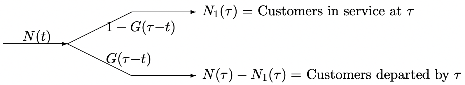
Note that as \(\tau \rightarrow \infty\), the integral in \ref{2.35} approaches the mean of the service time distribution (i.e., it is the integral of the complementary distribution function, \(1-G(t)\), of the service time). This means that in steady state (as \(\tau \rightarrow \infty\)), the distribution of the number in service at \(\tau\) depends on the service time distribution only through its mean. This example can be used to model situations such as the number of phone calls taking place at a given epoch. This requires arrivals of new calls to be modeled as a Poisson process and the holding time of each call to be modeled as a random variable independent of other holding times and of call arrival times. Finally, as shown in Figure 2.8, we can regard \(\left\{N_{1}(t) ; 0<t \leq \tau\right\}\) as a splitting of the arrival process \(\{N(t) ; t>0\}\). By the same type of argument as in Section 2.3, the number of customers who have completed service by time \(\tau\) is independent of the number still in service.

---

⁹We assume that \(\lambda(t)\) is right continuous, i.e., that for each \(t\), \(\lambda(t)\) is the limit of \(\lambda(t+\epsilon)\) as \(\epsilon\) approaches 0 from above. This allows \(\lambda(t)\) to contain discontinuities, as illustrated in Figure 2.7, but follows the convention that the value of the function at the discontinuity is the limiting value from the right. This convention is required in \ref{2.29} to talk about the distribution of arrivals just to the right of time \(t\).