2.5: Conditional Arrival Densities and Order Statistics

A diverse range of problems involving Poisson processes are best tackled by conditioning on a given number \(n\) of arrivals in the interval \((0, t]\), i.e., on the event \(N(t)=n\). Because of the incremental view of the Poisson process as independent and stationary arrivals in each incremental interval of the time axis, we would guess that the arrivals should have some sort of uniform distribution given \(N(t)=n\). More precisely, the following theorem shows that the joint density of \(\boldsymbol{S}^{(n)}=\left(S_{1}, S_{2}, \ldots, S_{n}\right)\) given \(N(t)=n\) is uniform over the region \(0<S_{1}<S_{2}<\cdots<S_{n}<t\).

Theorem 2.5.1

Let \(f_{S^{(n)} \mid N(t)}\left(\boldsymbol{s}^{(n)} \mid n\right)\) be the joint density of \(\boldsymbol{S}^{(n)}\) conditional on \(N(t)=n\). This density is constant over the region \(0<s_{1}<\cdots<s_{n}<t\) and has the value

\[f_{\boldsymbol{S}^{(n)} \mid N(t)}\left(\boldsymbol{s}^{(n)} \mid n\right)=\frac{n !}{t^{n}}\label{2.37} \]

Two proofs are given, each illustrative of useful techniques

Proof

Proof 1: Recall that the joint density of the first \(n+1\) arrivals \(\boldsymbol{S}^{(n+1)}=\left(S_{1} \ldots, S_{n}, S_{n+1}\right)\) with no conditioning is given in (2.15). We first use Bayes law to calculate the joint density of \(\boldsymbol{S}^{(n+1)}\) conditional on \(N(t)=n\).

\(\mathrm{f}_{\boldsymbol{S}^{(n+1)} \mid N(t)}\left(\boldsymbol{s}^{(n+1)} \mid n\right) \mathrm{p}_{N(t)}(n)=\mathbf{p}_{N(t) \mid \boldsymbol{S}^{(n+1)}}\left(n \mid \boldsymbol{s}^{(n+1)}\right) \mathrm{f}_{\boldsymbol{S}^{(n+1)}}\left(\boldsymbol{s}^{(n+1)}\right)\)

Note that \(N(t)=n\) if and only if \(S_{n} \leq t\) and \(S_{n+1}>t\). Thus \(\mathbf{p}_{N(t) \mid \boldsymbol{S}^{(n+1)}}\left(n \mid \boldsymbol{s}^{(n+1)}\right)\) is 1 if \(S_{n} \leq t\) and \(S_{n+1}>t\) and is 0 otherwise. Restricting attention to the case \(N(t)=n\), \(S_{n} \leq t\) and \(S_{n+1}>t\),

\[\begin{aligned}
{ }_{S^{(n+1)} \mid N(t)}\left(\boldsymbol{s}^{(n+1)} \mid n\right) &=\frac{\mathrm{f}_{\boldsymbol{S}^{(n+1)}}\left(\boldsymbol{s}^{(n+1)}\right)}{\mathrm{p}_{N(t)}(n)} \\
&=\frac{\lambda^{n+1} \exp \left(-\lambda s_{n+1}\right)}{(\lambda t)^{n} \exp (-\lambda t) / n !} \\
&=\frac{n ! \lambda \exp \left(-\lambda\left(s_{n+1}-t\right)\right.}{t^{n}}
\end{aligned}\label{2.38} \]

This is a useful expression, but we are interested in \(\boldsymbol{S}^{(n)}\) rather than \(\boldsymbol{S}^{(n+1)}\). Thus we break up the left side of \ref{2.38} as follows:

\(f_{\boldsymbol{S}^{(n+1)} \mid N(t)}\left(\boldsymbol{s}^{(n+1)} \mid n\right)=\mathrm{f}_{\boldsymbol{S}^{(n)} \mid N(t)}\left(\boldsymbol{s}^{(n)} \mid n\right) \mathrm{f}_{S_{n+1} \mid \boldsymbol{S}^{(n)} N(t)}\left(s_{n+1} \mid \boldsymbol{s}^{(n)}, n\right)\)

Conditional on \(N(t)=n, S_{n+1}\) is the first arrival epoch after \(t\), which by the memoryless property is independent of \(\boldsymbol{S}^{(n)}\). Thus that final term is simply \(\lambda \exp \left(-\lambda\left(s_{n+1}-t\right)\right)\) for \(s_{n+1}>t\). Substituting this into (2.38), the result is (2.37).

Proof 2: This alternative proof derives \ref{2.37} by looking at arrivals in very small increments of size \(\delta\) (see Figure 2.9). For a given \(t\) and a given set of \(n\) times, \(0<s_{1}<\cdots,<s_{n}<t\), we calculate the probability that there is a single arrival in each of the intervals \(\left(s_{i}, s_{i}+\delta\right], 1 \leq i \leq n\) and no other arrivals in the interval \((0, t]\). Letting \(A(\delta)\) be this event,

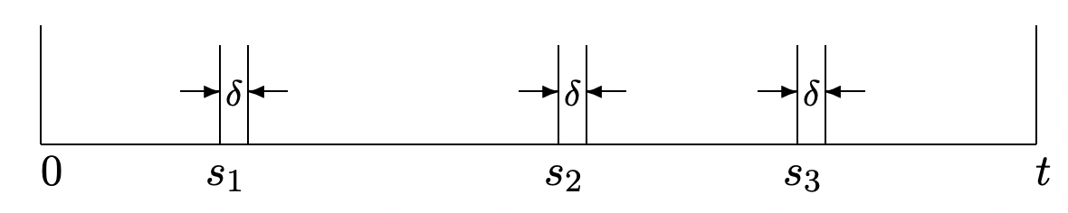Figure 2.9: Intervals for arrival density.

\(\operatorname{Pr}\{A(\delta)\}=\mathbf{p}_{N\left(s_{1}\right)}(0) \mathbf{p}_{\widetilde{N}\left(s_{1}, s_{1}+\delta\right)}(1) \mathbf{p}_{\tilde{N}\left(s_{1}+\delta, s_{2}\right)}(0) \mathbf{p}_{\tilde{N}\left(s_{2}, s_{2}+\delta\right)}(1) \cdots \mathbf{p}_{\tilde{N}\left(s_{n}+\delta, t\right)}(0)\)

The sum of the lengths of the above intervals is \(t\), so if we represent \(\mathbf{p}_{\tilde{N}\left(s_{i}, s_{i}+\delta\right)}(1)\) as \(\lambda \delta \exp (-\lambda \delta)+o(\delta)\) for each \(i\), then

\(\operatorname{Pr}\{A(\delta)\}=(\lambda \delta)^{n} \exp (-\lambda t)+\delta^{n-1} o(\delta)\)

The event \(A(\delta)\) can be characterized as the event that, first, \(N(t)=n\) and, second, that the \(n\) arrivals occur in \(\left(s_{i}, s_{i}+\delta\right]\) for \(1 \leq i \leq n\). Thus we conclude that

\(f_{S^{(n)} \mid N(t)}\left(\boldsymbol{s}^{(n)}\right)=\lim _{\delta \rightarrow 0} \frac{\operatorname{Pr}\{A(\delta)\}}{\delta^{n} \mathbf{p}_{N(t)}(n)}\)

which simplifies to (2.37).

The joint density of the interarrival intervals, \(\boldsymbol{X}^{(n)}=\left(X_{1} \ldots, X_{n}\right)\) given \(N(t)=n\) can be found directly from Theorem 2.5.1 simply by making the linear transformation \(X_{1}=S_{1}\) and \(X_{i}=S_{i}-S_{i-1}\) for \(2 \leq i \leq n\). The density is unchanged, but the constraint region transforms into \(\sum_{i=1}^{n} X_{i}<t\) with \(X_{i}>0\) for \(1 \leq i \leq n\) (see Figure 2.10).

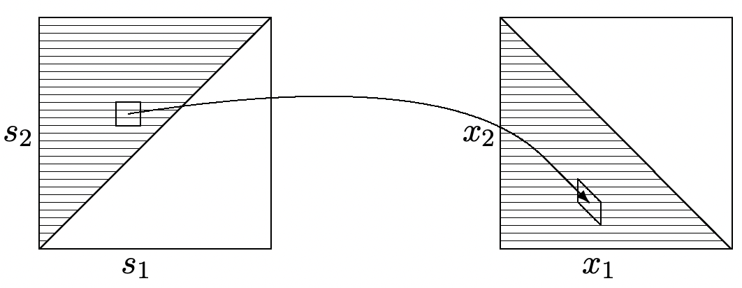Figure 2.10: Mapping from arrival epochs to interarrival times. Note that incremental cubes in the arrival space map to parallelepipeds of the same volume in the interarrival space.

\[f_{\boldsymbol{X}^{(n)} \mid N(t)}\left(\boldsymbol{x}^{(n)} \mid n\right)=\frac{n !}{t^{n}} \quad \text { for } \boldsymbol{X}^{(n)}>0, \sum_{i=1}^{n} X_{i}<t\label{2.39} \]

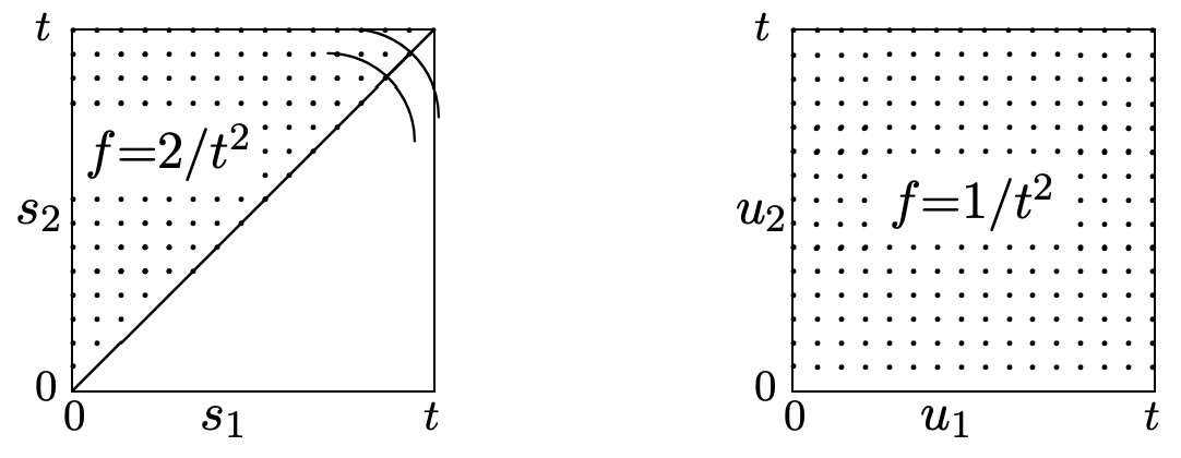
It is also instructive to compare the joint distribution of \(\boldsymbol{S}^{(n)}\) conditional on \(N(t)=n\) with the joint distribution of \(n\) IID uniformly distributed random variables, \(\boldsymbol{U}^{(n)}=\left(U_{1}, \ldots, U_{n}\right)\) on \((0, t]\). For any point \(\boldsymbol{U}^{(n)}=\boldsymbol{u}^{(n)}\), this joint density is

\(f_{U^{(n)}}\left(\boldsymbol{u}^{(n)}\right)=1 / t^{n} \text { for } 0<u_{i} \leq t, 1 \leq i \leq n\)

Both \(\mathbf{f}_{\boldsymbol{S}^{(n)}}\) and \(f_{\boldsymbol{U}^{(n)}}\) are uniform over the volume of n-space where they are non-zero, but as illustrated in Figure 2.11 for \(n=2\), the volume for the latter is \(n !\) times larger than the volume for the former. To explain this more fully, we can define a set of random variables \(S_{1}, \ldots, S_{n}\) not as arrival epochs in a Poisson process, but rather as the order statistics function of the IID uniform variables \(U_{1}, \ldots, U_{n}\); that is

\(S_{1}=\min \left(U_{1}, \ldots, U_{n}\right) ; S_{2}=2^{\text {nd }} \text { smallest }\left(U_{1}, \ldots, U_{n}\right) ; \text { etc. }\)

Figure 2.11: Density for the order statistics of an IID 2-dimensional uniform distribution. Note that the square over which \(f_{U^{(2)}}\) is non-zero contains one triangle where \(u_{2}>u_{1}\) and another of equal size where \(u_{1}>u_{2}\). Each of these maps, by a permutation mapping, to the single triangle where \(s_{2}>s_{1}\).

The \(n\)-cube is partitioned into \(n !\) regions, one where \(u_{1}<u_{2}<\cdots<u_{n}\). For each permutation \(\pi(i)\) of the integers 1 to \(n\), there is another region¹⁰ where \(u_{\pi(1)}<u_{\pi(2)}<\dots<u_{\pi(n)}\). By symmetry, each of these regions has the same volume, which then must be \(1 / n !\) of the volume \(t^{n}\) of the \(n\)-cube.

All of these \(n !\) regions map to the same region of ordered values. Thus these order statistics have the same joint probability density function as the arrival epochs \(S_{1}, \ldots, S_{n}\) conditional on \(N(t)=n\). Anything we know (or can discover) about order statistics is valid for arrival epochs given \(N(t)=n\) and vice versa.¹¹

Next we want to find the marginal distribution functions of the individual \(S_{i}\), conditional on \(N(t)=n\). Starting with \(S_{1}\), and viewing it as the minimum of the IID uniformly distributed variables \(U_{1}, \ldots, U_{n}\), we recognize that \(S_{1}>\tau\) if and only if \(U_{i}>\tau\) for all \(i, 1 \leq i \leq n\).

Thus,

\[\operatorname{Pr}\left\{S_{1}>\tau \mid N(t)=n\right\}=\left[\frac{t-\tau}{t}\right]^{n} \quad \text { for } 0<\tau \leq t\label{2.40} \]

For \(S_{2}\) to \(S_{n}\), the density is slightly simpler in appearance than the distribution function. To find \(\mathrm{f}_{S_{i} \mid N(t)}\left(s_{i} \mid n\right)\), look at \(n\) uniformly distributed rv’s in \((0, t]\). The probability that one of these lies in the interval \(\left(s_{i}, s_{i}+d t\right]\) is \((n d t) / t\). Out of the remaining \(n-1\), the probability that \(i-1\) lie in the interval \(\left(0, s_{i}\right]\) is given by the binomial distribution with probability of success \(s_{i} / t\). Thus the desired density is

\[\begin{aligned}
\mathrm{f}_{S_{i} \mid N(t)}(x \mid n) d t &=\frac{s_{i}^{i-1}\left(t-s_{i}\right)^{n-i}(n-1) !}{t^{n-1}(n-i) !(i-1) !} \quad \frac{n d t}{t} \\
\mathrm{f}_{S_{i} \mid N(t)}\left(s_{i} \mid n\right) &=\frac{s_{i}^{i-1}\left(t-s_{i}\right)^{n-i} n !}{t^{n}(n-i) !(i-1) !}
\end{aligned}\label{2.41} \]

It is easy to find the expected value of \(S_{1}\) conditional on \(N(t)=n\) by integrating the complementary distribution function in (2.40), getting

\[\mathrm{E}\left[S_{1} \mid N(t)=n\right]=\frac{t}{n+1}\label{2.42} \]

We come back later to find \(\mathrm{E}\left[S_{i} \mid N(t)=n\right]\) for \(2 \leq i \leq n\). First, we look at the marginal distributions of the interarrival intervals. Recall from \ref{2.39} that

\[f_{\boldsymbol{X}^{(n)} \mid N(t)}\left(\boldsymbol{x}^{(n)} \mid n\right)=\frac{n !}{t^{n}} \quad \text { for } \boldsymbol{X}^{(n)}>0, \sum_{i=1}^{n} X_{i}<t\label{2.43} \]

The joint density is the same for all points in the constraint region, and the constraint does not distinguish between \(X_{1}\) to \(X_{n}\). Thus \(X_{1}, \ldots, X_{n}\) must all have the same marginal distribution, and more generally the marginal distribution of any subset of the \(X_{i}\) can depend only on the size of the subset. We have found the distribution of \(S_{1}\), which is the same as \(X_{1}\), and thus

\[\operatorname{Pr}\left\{X_{i}>\tau \mid N(t)=n\right\}=\left[\frac{t-\tau}{t}\right]^{n} \quad \text { for } 1 \leq i \leq n \text { and } 0<\tau \leq t.\label{2.44} \]

\[\mathrm{E}\left[X_{i} \mid N(t)=n\right]=\frac{t}{n+1} \quad \text { for } 1 \leq i \leq n .\label{2.45} \]

From this, we see immediately that for \(1 \leq i \leq n\),

\[\mathrm{E}\left[S_{i} \mid N(t)=n\right]=\frac{i t}{n+1}\label{2.46} \]

One could go on and derive joint distributions of all sorts at this point, but there is one additional type of interval that must be discussed. Define \(X_{n+1}^{*}=t-S_{n}\) to be the interval from the largest arrival epoch before \(t\) to \(t\) itself. Rewriting (2.43),

\(f_{\boldsymbol{X}^{(n)} \mid N(t)}\left(\boldsymbol{x}^{(n)} \mid n\right)=\frac{n !}{t^{n}} \quad \text { for } \boldsymbol{X}^{(n)}>0, X_{n+1}^{*}>0, \sum_{i=1}^{n} X_{i}+X_{n+1}^{*}=t\)

The constraints above are symmetric in \(X_{1}, \ldots, X_{n}, X_{n+1}^{*}\), and, within the constraint region, the joint density of \(X_{1}, \ldots, X_{n}\) (conditional on \(N(t)=n\)) is uniform. Note that there is no joint density over \(X_{1}, \ldots, X_{n}, X_{n+1}^{*}\) condtional on \(n(t)=n\), since \(X_{n+1}^{*}\) is then a deterministic function of \(X_{1}, \ldots, X_{n}\). However, the density over \(X_{1}, \ldots, X_{n}\) can be replaced by a density over any other \(n\) rv’s out of \(X_{1}, \ldots, X_{n}, X_{n+1}^{*}\) by a linear transformation with unit determinant. Thus \(X_{n+1}^{*}\) has the same marginal distribution as each of the \(X_{i}\). This gives us a partial check on our work, since the interval \((0, t]\) is divided into \(n+1\) intervals of sizes \(X_{1}, X_{2}, \ldots, X_{n}, X_{n+1}^{*}\), and each of these has a mean size \(t /(n+1)\). We also see that the joint distribution function of any proper subset of \(X_{1}, X_{2}, \ldots X_{n}, X_{n+1}^{*}\) is independent of the order of the variables.

One important consequece of this is that we can look at a segment \((0, t]\) of a Poisson process either forward or backward in time and it ‘looks the same.’ Looked at backwards, the interarrival intervals are \(X_{n+1}^{*}, X_{n}, \ldots, X_{2}\). These intervals are IID, and \(X_{1}\) is then determined as \(t-X_{n+1}^{*}-X_{n}-\cdots-X_{2}\). We will not make any particular use of this property here, but we will later explore this property of time-reversibility for other types of processes. For Poisson processes, this reversibility is intuitively obvious from the stationary and independent properties. It is less obvious how to express this condition by equations, but that is not really necessary at this point.

---

Reference

¹⁰As usual, we are ignoring those points where \(u_{i}=u_{j}\) for some \(i\), \(j\), since the set of such points has 0 probability.

¹¹There is certainly also the intuitive notion, given \(n\) arrivals in \((0, t]\), and given the stationary and independent increment properties of the Poisson process, that those \(n\) arrivals can be viewed as uniformly distributed. One way to view this is to visualize the Poisson process as the sum of a very large number \(k\) of independent processes of rate \(\lambda / k\) each. Then, given \(N(t)=n\), with \(k>>n\), there is negligible probability of more than one arrival from any one process, and for each of the n processes with arrivals, that arrival is uniformly distributed in \((0, t]\).