3.1: Introduction to Finite-state Markov Chains

The counting processes \(\{N(t) ; t>0\}\) described in Section 2.1.1 have the property that \(N(t)\) changes at discrete instants of time, but is defined for all real \(t>0\). The Markov chains to be discussed in this chapter are stochastic processes defined only at integer values of time, \(n=0,1, \ldots\). At each integer time \(n \geq 0\), there is an integer-valued random variable (rv) \(X_{n}\), called the state at time \(n\), and the process is the family of rv’s \(\left\{X_{n} ; n \geq 0\right\}\). We refer to these processes as integer-time processes. An integer-time process \(\left\{X_{n} ; n \geq 0\right\}\) can also be viewed as a process \(\{X(t) ; t \geq 0\}\) defined for all real \(t\) by taking \(X(t)=X_{n}\) for \(n \leq t<n+1\), but since changes occur only at integer times, it is usually simpler to view the process only at those integer times.

In general, for Markov chains, the set of possible values for each rv \(X_{n}\) is a countable set \(\mathcal{S}\). If \(\mathcal{S}\) is countably infinite, it is usually taken to be \(\mathcal{S}=\{0,1,2, \ldots\}\), whereas if \(\mathcal{S}\) is finite, it is usually taken to be \(\mathcal{S}=\{1, \ldots, \mathrm{M}\}\). In this chapter (except for Theorems 3.2.2 and 3.2.3), we restrict attention to the case in which \(\mathcal{S}\) is finite, i.e., processes whose sample functions are sequences of integers, each between 1 and M. There is no special significance to using integer labels for states, and no compelling reason to include 0 for the countably infinite case and not for the finite case. For the countably infinite case, the most common applications come from queueing theory, where the state often represents the number of waiting customers, which might be zero. For the finite case, we often use vectors and matrices, where positive integer labels simplify the notation. In some examples, it will be more convenient to use more illustrative labels for states.

Definition 3.1.1

A Markov chain is an integer-time process, \(\left\{X_{n}, n \geq 0\right\}\) for which the sample values for each rv \(X_{n}\), \(n \geq 1\), lie in a countable set \(\mathcal{S}\) and depend on the past only through the most recent rv \(X_{n-1}\). More specifically, for all positive integers \(n\), and for all \(i, j, k, \ldots, m\) in \(\mathcal{S}\),

\[\operatorname{Pr}\left\{X_{n}=j \mid X_{n-1}=i, X_{n-2}=k, \ldots, X_{0}=m\right\}=\operatorname{Pr}\left\{X_{n}=j \mid X_{n-1}=i\right\}\label{3.1} \]

Furthermore, \(\operatorname{Pr}\left\{X_{n}=j \mid X_{n-1}=i\right\}\) depends only on \(i\) and j (not \(n\)) and is denoted by

\[\operatorname{Pr}\left\{X_{n}=j \mid X_{n-1}=i\right\}=P_{i j}\label{3.2} \]

The initial state \(X_{0}\) has an arbitrary probability distribution. A finite-state Markov chain is a Markov chain in which \(\mathcal{S}\) is finite.

Equations such as \ref{3.1} are often easier to read if they are abbreviated as

\(\operatorname{Pr}\left\{X_{n} \mid X_{n-1}, X_{n-2}, \ldots, X_{0}\right\}=\operatorname{Pr}\left\{X_{n} \mid X_{n-1}\right\}\)

This abbreviation means that equality holds for all sample values of each of the rv’s. i.e., it means the same thing as (3.1).

The rv \(X_{n}\) is called the state of the chain at time \(n\). The possible values for the state at time \(n\), namely \(\{1, \ldots, \mathrm{M}\}\) or \(\{0,1, \ldots\}\) are also generally called states, usually without too much confusion. Thus \(P_{i j}\) is the probability of going to state \(j\) given that the previous state is \(i\); the new state, given the previous state, is independent of all earlier states. The use of the word state here conforms to the usual idea of the state of a system — the state at a given time summarizes everything about the past that is relevant to the future.

Definition 3.1.1 is used by some people as the definition of a homogeneous Markov chain. For them, Markov chains include more general cases where the transition probabilities can vary with n. Thus they replace \ref{3.1} and \ref{3.2} by

\[\operatorname{Pr}\left\{X_{n}=j \mid X_{n-1}=i, X_{n-2}=k, \ldots, X_{0}=m\right\}=\operatorname{Pr}\left\{X_{n}=j \mid X_{n-1}=i\right\}=P_{i j}(n)\label{3.3} \]

We will call a process that obeys (3.3), with a dependence on n, a non-homogeneous Markov chain. We will discuss only the homogeneous case, with no dependence on n, and thus restrict the definition to that case. Not much of general interest can be said about nonhomogeneous chains.¹

An initial probability distribution for \(X_{0}\), combined with the transition probabilities \(\left\{P_{i j}\right\}\) (or \(\left\{P_{i j}(n)\right\}\)) for the non-homogeneous case), define the probabilities for all events in the Markov chain.

Markov chains can be used to model an enormous variety of physical phenomena and can be used to approximate many other kinds of stochastic processes such as the following example:

Exercise 3.1.1

Consider an integer process \(\left\{Z_{n} ; n \geq 0\right\}\) where the \(Z_{n}\) are finite integervalued rv’s as in a Markov chain, but each \(Z_{n}\) depends probabilistically on the previous \(k\) rv’s, \(Z_{n-1}, Z_{n-2}, \ldots, Z_{n-k}\). In other words, using abbreviated notation,

\[\operatorname{Pr}\left\{Z_{n} \mid Z_{n-1}, Z_{n-2}, \ldots, Z_{0}\right\}=\operatorname{Pr}\left\{Z_{n} \mid Z_{n-1}, \ldots Z_{n-k}\right\}\label{3.4} \]

Answer

We now show how to view the condition on the right side of (3.4), i.e., \(\left(Z_{n-1}, Z_{n-2}, \ldots, Z_{n-k}\right)\) as the state of the process at time \(n-1\). We can rewrite \ref{3.4} as

\(\operatorname{Pr}\left\{Z_{n}, Z_{n-1}, \ldots, Z_{n-k+1} \mid Z_{n-1}, \ldots, Z_{0}\right\}=\operatorname{Pr}\left\{Z_{n}, \ldots, Z_{n-k+1} \mid Z_{n-1}, \ldots Z_{n-k}\right\}\)

since, for each side of the equation, any given set of values for \(Z_{n-1}, \ldots, Z_{n-k+1}\) on the right side of the conditioning sign specifies those values on the left side. Thus if we define \(X_{n-1}=\left(Z_{n-1}, \ldots, Z_{n-k}\right)\) for each \(n\), this simplifies to

\(\operatorname{Pr}\left\{X_{n} \mid X_{n-1}, \ldots, X_{k-1}\right\}=\operatorname{Pr}\left\{X_{n} \mid X_{n-1}\right\}\)

We see that by expanding the state space to include k-tuples of the rv’s \(Z_{n}\), we have converted the \(k\) dependence over time to a unit dependence over time, i.e., a Markov process is defined using the expanded state space.

Note that in this new Markov chain, the initial state is \(X_{k-1}=\left(Z_{k-1}, \ldots, Z_{0}\right)\), so one might want to shift the time axis to start with \(X_{0}\).

Markov chains are often described by a directed graph (see Figure 3.1 a). In this graphical representation, there is one node for each state and a directed arc for each non-zero transition probability. If \(P_{i j}=0\), then the arc from node \(i\) to node \(j\) is omitted, so the difference between zero and non-zero transition probabilities stands out clearly in the graph. The classification of states, as discussed in Section 3.2, is determined by the set of transitions with non-zero probabilities, and thus the graphical representation is ideal for that topic.

A finite-state Markov chain is also often described by a matrix \([P]\) (see Figure 3.1 b). If the chain has M states, then \([P]\) is an M by M matrix with elements \(P_{i j}\). The matrix representation is ideally suited for studying algebraic and computational issues.

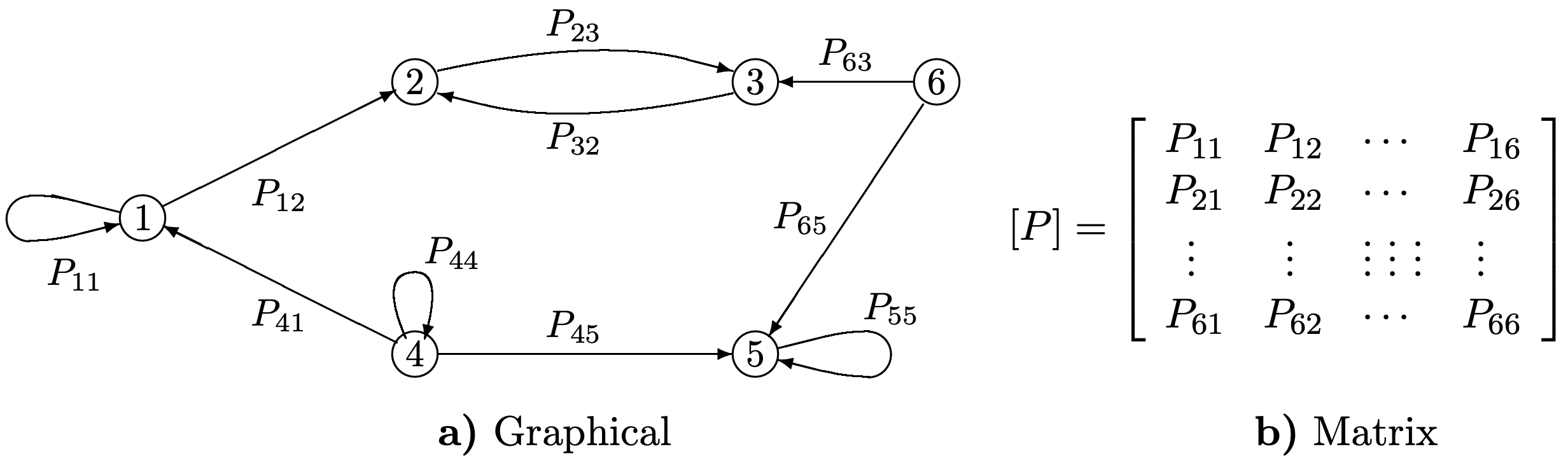
Figure 3.1: Graphical and Matrix Representation of a 6 state Markov Chain; a directed arc from \(i\) to \(j\) is included in the graph if and only if (iff) \(P_{i j}>0\).

---

Reference

¹On the other hand, we frequently find situations where a small set of rv’s, say \(W, X, Y, Z\) satisfy the Markov condition that \(\operatorname{Pr}\{Z \mid Y, X, W\}=\operatorname{Pr}\{Z \mid Y\}\) and \(\operatorname{Pr}\{Y \mid X, W\}=\operatorname{Pr}\{Y \mid X\}\) but where the conditional distributions \(\operatorname{Pr}\{Z \mid Y\}\) and \(\operatorname{Pr}\{Y \mid X\}\) are unrelated. In other words, Markov chains imply homogeniety here, whereas the Markov condition does not.