3.2: Classification of States

This section, except where indicated otherwise, applies to Markov chains with both finite and countable state spaces. We start with several definitions.

Definition: 3.2.1

An (n-step) walk is an ordered string of nodes, (i0,i1, . . .in), n ≥ 1, in which there is a directed arc from \(i_{m−1}\) to \(i_m\) for each m, 1 ≤ m ≤ n. A path is a walk in which no nodes are repeated. A cycle is a walk in which the first and last nodes are the same and no other node is repeated.

Note that a walk can start and end on the same node, whereas a path cannot. Also the number of steps in a walk can be arbitrarily large, whereas a path can have at most M − 1 steps and a cycle at most M steps for a finite-state Markov chain with |S| = M.

Definition 3.2.2

A state \(j\) is accessible from \(i\) (abbreviated as \(i_j\)) if there is a walk in the graph from \(i\) to \(j\).

For example, in Figure 3.1(a), there is a walk from node 1 to node 3 (passing through node 2), so state 3 is accessible from 1. There is no walk from node 5 to 3, so state 3 is not accessible from 5. State 2 is accessible from itself, but state 6 is not accessible from itself. To see the probabilistic meaning of accessibility, suppose that a walk \(i_{0}, i_{1}, \ldots i_{n}\) exists from node \(i_{0}\) to \(i_{n}\). Then, conditional on \(X_{0}=i_{0}\), there is a positive probability, \(P_{i_{0} i_{1}}\), that \(X_{1}=i_{1}\), and consequently (since \(P_{i_{1} i_{2}}>0\)), there is a positive probability that \(X_{2}=i_{2}\). Continuing this argument, there is a positive probability that \(X_{n}=i_{n}\), so that \(\operatorname{Pr}\left\{X_{n}=i_{n} \mid X_{0}=i_{0}\right\}>0\). Similarly, if \(\operatorname{Pr}\left\{X_{n}=i_{n} \mid X_{0}=i_{0}\right\}>0\), then an \(n\)-step walk from \(i_{0}\) to \({i}_{n}\) must exist. Summarizing, \(i \rightarrow j\) if and only if (iff) \(\operatorname{Pr}\left\{X_{n}=j \mid X_{0}=i\right\}>0\) for some \(n \geq 1\). We denote \(\operatorname{Pr}\left\{X_{n}=j \mid X_{0}=i\right\}\) by \(P_{i j}^{n}\). Thus, for \(n \geq 1, P_{i j}^{n}>0\) if and only if the graph has an \(n\) step walk from \(i\) to \(j\) (perhaps visiting the same node more than once). For the example in Figure 3.1(a), \(P_{13}^{2}=P_{12} P_{23}>0\). On the other hand, \(P_{53}^{n}=0\) for all \(n \geq 1\). An important relation that we use often in what follows is that if there is an \(n\)-step walk from state \(i\) to \(j\) and an \(m\)-step walk from state \(j\) to \(k\), then there is a walk of \(m + n\) steps from \(i\) to \(k\). Thus

\[P_{i j}^{n}>0 \text { and } P_{j k}^{m}>0 \quad \text { imply } \quad P_{i k}^{n+m}>0\label{3.5} \]

This also shows that

\[i \rightarrow j \text { and } \mathrm{j} \rightarrow \mathrm{k} \quad\text { imply } \quad\mathrm{i} \rightarrow \mathrm{k}\label{3.6} \]

Definition 3.2.3

Two distinct states \(i\) and \(j\) communicate (abbreviated \(i \leftrightarrow j\)) if \(i\) is accessible from \(j\) and \(j\) is accessible from \(i\).

An important fact about communicating states is that if \(i \leftrightarrow j\) and \(m \leftrightarrow j\) then \(i \leftrightarrow m\). To see this, note that \(i \leftrightarrow j\) and \(m \leftrightarrow j\) imply that \(i \rightarrow j\) and j \(\rightarrow m\), so that \(i \rightarrow m\). Similarly, \(m \rightarrow i\), so \(i \leftrightarrow m\).

Definition 3.2.4

\(A\) class \(C\) of states is a non-empty set of states such that each \(i \in \mathcal{C}\) communicates with every other state \(j \in \mathcal{C}\) and communicates with no \(j \notin \mathcal{C}\).

For the example of Figure 3.1(a), {2, 3} is one class of states, {1}, {4}, {5}, and {6} are the other classes. Note that state 6 does not communicate with any other state, and is not even accessible from itself, but the set consisting of {6} alone is still a class. The entire set of states in a given Markov chain is partitioned into one or more disjoint classes in this way.

Definition 3.2.5

For finite-state Markov chains, a recurrent state is a state \(i\) that is accessible from all states that are accessible from \(i\) (\(i\) is recurrent if \(i \rightarrow j\) implies that \(j \rightarrow i\). A transient state is a state that is not recurrent.

Recurrent and transient states for Markov chains with a countably-infinite state space will be defined in Chapter 5.

According to the definition, a state \(i\) in a finite-state Markov chain is recurrent if there is no possibility of going to a state \(j\) from which there can be no return. As we shall see later, if a Markov chain ever enters a recurrent state, it returns to that state eventually with probability 1, and thus keeps returning infinitely often (in fact, this property serves as the definition of recurrence for Markov chains without the finite-state restriction). A state \(i\) is transient if there is some j that is accessible from i but from which there is no possible return. Each time the system returns to \(i\), there is a possibility of going to \(j\); eventually this possibility will occur with no further returns to \(i\).

Theorem 3.2.1

For finite-state Markov chains, either all states in a class are transient or all are recurrent.²

Proof

Assume that state \(i\) is transient (i.e., for some \(j\), \(i \rightarrow j\) but \(j \not \rightarrow i\)) and suppose that \(i\) and \(m\) are in the same class (i.e., \(i \leftrightarrow m\)). Then \(m \rightarrow i\) and \(i \rightarrow j\), so \(m \rightarrow j\). Now if \(j \rightarrow m\), then the walk from \(j\) to m could be extended to \(i\); this is a contradiction, and therefore there is no walk from \(j\) to \(m\), and \(m\) is transient. Since we have just shown that all nodes in a class are transient if any are, it follows that the states in a class are either all recurrent or all transient.

For the example of Figure 3.1(a), {2, 3} and {5} are recurrent classes and the other classes are transient. In terms of the graph of a Markov chain, a class is transient if there are any directed arcs going from a node in the class to a node outside the class. Every finite-state Markov chain must have at least one recurrent class of states (see Exercise 3.2), and can have arbitrarily many additional classes of recurrent states and transient states.

States can also be classified according to their periods (see Figure 3.2). For \(X_{0}=2 \) in Figure 3.2(a), \(X_{n}\) must be 2 or 4 for \(n\) even and 1 or 3 for n odd. On the other hand, if \(X_{0}\) is 1 or 3, then \(X_{n}\) is 2 or 4 for \(n\) odd and 1 or 3 for \(n\) even. Thus the effect of the starting state never dies out. Figure 3.2(b) illustrates another example in which the memory of the starting state never dies out. The states in both of these Markov chains are said to be periodic with period 2. Another example of periodic states are states 2 and 3 in Figure 3.1(a).

Definition 3.2.6: Greatest Common Divisor

The period of a state \(i\), denoted \(d(i)\), is the greatest common divisor (gcd) of those values of \(n\) for which \(P_{i i}^{n}>0\). If the period is 1, the state is aperiodic, and if the period is 2 or more, the state is periodic.

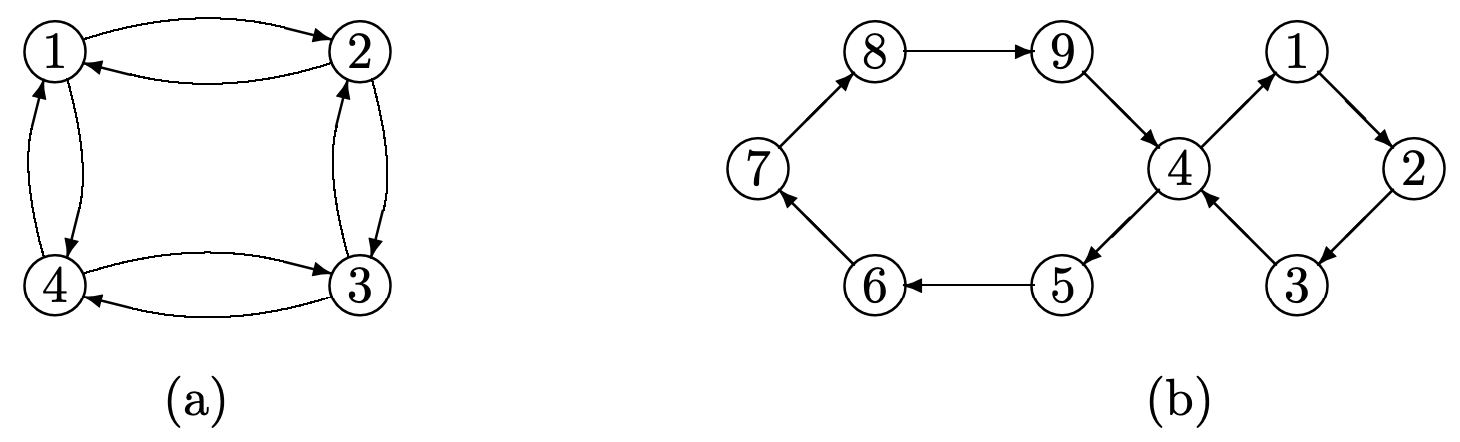Figure 3.2: Periodic Markov Chains

For example, in Figure 3.2(a), \(P_{11}^{n}>0\) for \(n=2,4,6, \ldots\) Thus \(d(1)\), the period of state 1, is two. Similarly, \(d(i)=2\) for the other states in Figure 3.2(a). For Figure 3.2(b), we have \(P_{11}^{n}>0\) for \(n=4,8,10,12, \ldots\); thus \(d(1)=2\), and it can be seen that \(d(i)=2\) for all the states. These examples suggest the following theorem.

Theorem 3.2.2

For any Markov chain (with either a finite or countably infinite number of states), all states in the same class have the same period.

Proof

Let \(i\) and \(j\) be any distinct pair of states in a class \(\mathcal{C}\). Then \(i \leftrightarrow j\) and there is some \(r\) such that \(P_{i j}^{r}>0\) and some \(s\) such that \(P_{j i}^{s}>0\). Since there is a walk of length \(r+s\) going from \(i\) to \(j\) and back to \(i\), \(r+s\) must be divisible by \(d(i)\). Let \(t\) be any integer such that \(P_{j j}^{t}>0\). Since there is a walk of length \(r+t+s\) from \(i\) to \(j\), then back to \(j\), and then to \(i\), \(r+t+s\) is divisible by \(d(i)\), and thus \(t\) is divisible by \(d(i)\). Since this is true for any \(t\) such that \(P_{j j}^{t}>0\), \(d(j)\) is divisible by \(d(i)\). Reversing the roles of \(i\) and \(j\), \(d(i)\) is divisible by \(d(j)\), so \(d(i)=d(j)\).

Since the states in a class \(\mathcal{C}\) all have the same period and are either all recurrent or all transient, we refer to \(\mathcal{C}\) itself as having the period of its states and as being recurrent or transient. Similarly if a Markov chain has a single class of states, we refer to the chain as having the corresponding period.

Theorem 3.2.3

If a recurrent class \(\mathcal{C}\) in a finite-state Markov chain has period \(d\), then the states in \(\mathcal{C}\) can be partitioned into \(d\) subsets, \(\mathcal{S}_{1}, \mathcal{S}_{2}, \ldots, \mathcal{S}_{d}\), in such a way that all transitions from \(\mathcal{S}_{1}\) go to \(\mathcal{S}_{2}\), all from \(\mathcal{S}_{2}\) go to \(\mathcal{S}_{3}\), and so forth up to \(\mathcal{S}_{m-1}\) to \(\mathcal{S}_{m}\). Finally, all transitions from \(\mathcal{S}_{m}\) go to \(\mathcal{S}_{1}\).

Proof

See Figure 3.3 for an illustration of the theorem. For a given state in \(\mathcal{C}\), say state 1, define the sets \(\mathcal{S}_{1}, \ldots, \mathcal{S}_{d}\) by

\[\mathcal{S}_{m}=\left\{j: P_{1 j}^{n d+m}>0 \text { for some } n \geq 0\right\} ; \quad 1 \leq m \leq d\label{3.7} \]

For each \(j \in \mathcal{C}\), we first show that there is one and only one value of \(m\) such that \(j \in \mathcal{S}_{m}\). Since \(1 \leftrightarrow j\), there is some \(r\) for which \(P_{1 j}^{r}>0\) and some \(s\) for which \(P_{j 1}^{s}>0\). Thus there is a walk from 1 to 1 (through \(j\)) of length \(r+s\), so \(r+s\) is divisible by \(d\). For the given \(r\), let \(m\), \(1 \leq m \leq d\), satisfy \(r=m+n d\), where \(n\) is an integer. From (3.7), \(j \in \mathcal{S}_{m}\). Now let \(r^{\prime}\) be any other integer such that \(P_{1 j}^{r^{\prime}}>0\). Then \(r^{\prime}+s\) is also divisible by \(d\), so that \(r^{\prime}-r\) is divisible by \(d\). Thus \(r^{\prime}=m+n^{\prime} d\) for some integer \(n^{\prime}\) and that same \(m\). Since \(r^{\prime}\) is any integer such that \(P_{1 j}^{r^{\prime}}>0, j\) is in \(\mathcal{S}_{m}\) for only that one value of \(m\). Since \(j\) is arbitrary, this shows that the sets \(\mathcal{S}_{m}\) are disjoint and partition \(\mathcal{C}\).

Finally, suppose \(j \in \mathcal{S}_{m}\) and \(P_{j k}>0\). Given a walk of length \(r=n d+m\) from state 1 to \(j\), there is a walk of length \(n d+m+1\) from state 1 to \(k\). It follows that if \(m<d\), then \(k \in \mathcal{S}_{m+1}\) and if \(m=d\), then \(k \in \mathcal{S}_{1}\), completing the proof.

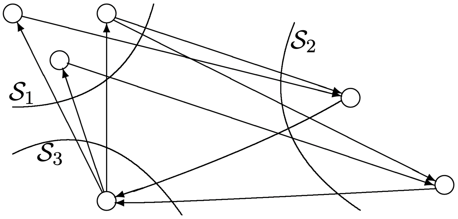
Figure 3.3: Structure of a periodic Markov chain with \(d=3\). Note that transitions only go from one subset \(\mathcal{S}_{m}\) to the next subset \(\mathcal{S}_{m+1}\) (or from \(\mathcal{S}_{d}\) to \(\mathcal{S}_{1}\)).

We have seen that each class of states (for a finite-state chain) can be classified both in terms of its period and in terms of whether or not it is recurrent. The most important case is that in which a class is both recurrent and aperiodic.

Definition 3.2.7

For a finite-state Markov chain, an ergodic class of states is a class that is both recurrent and aperiodic³. A Markov chain consisting entirely of one ergodic class is called an ergodic chain.

We shall see later that these chains have the desirable property that \(P_{i j}^{n}\) becomes independent of the starting state \(i\) as \(n \rightarrow \infty\). The next theorem establishes the first part of this by showing that \(P_{i j}^{n}>0\) for all \(i\) and \(j\) when \(n\) is sufficiently large. A guided proof is given in Exercise 3.5.

Theorem 3.2.4

For an ergodic \(M\) state Markov chain, \(P_{i j}^{m}>0\) for all \(i\), \(j\), and all \(m \geq (M-1)^2+1\).

Proof

Figure 3.4 illustrates a situation where the bound \((\mathrm{M}-1)^{2}+1\) is met with equality. Note that there is one cycle of length \(\mathrm{M}-1\) and the single node not on this cycle, node 1, is the unique starting node at which the bound is met with equality.

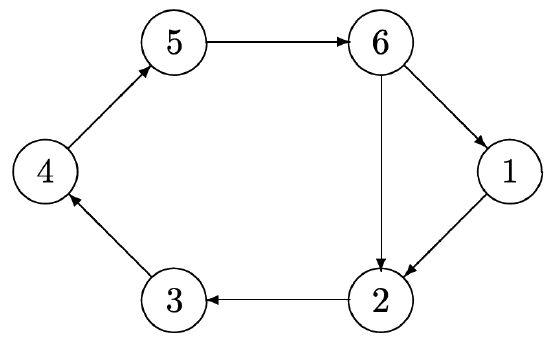
Figure 3.4: An ergodic chain with \(\mathrm{M}=6\) states in which \(P_{i j}^{m}>0\) for all \(m>(\mathrm{M}-1)^{2}\) and all \(i\), \(j\) but \(P_{11}^{(\mathrm{M}-1)^{2}}=0\) The figure also illustrates that an M state Markov chain must have a cycle with M − 1 or fewer nodes. To see this, note that an ergodic chain must have cycles, since each node must have a walk to itself, and subcycles of repeated nodes can be omitted from that walk, converting it into a cycle. Such a cycle might have M nodes, but a chain with only an M node cycle would be periodic. Thus some nodes must be on smaller cycles, such as the cycle of length 5 in the figure.

---

Reference

²As shown in Chapter 5, this theorem is also true for Markov chains with a countably infinite state space, but the proof given here is inadequate. Also recurrent classes with a countably infinite state space are further classified into either positive-recurrent or null-recurrent, a distinction that does not appear in the finite-state case.

³For Markov chains with a countably infinite state space, ergodic means that the states are positiverecurrent and aperiodic (see Chapter 5, Section 5.1).