3.3: The Matrix Representation

The matrix \([P]\) of transition probabilities of a Markov chain is called a stochastic matrix; that is, a stochastic matrix is a square matrix of nonnegative terms in which the elements in each row sum to 1. We first consider the n step transition probabilities \(P_{i j}^{n}\) in terms of \(\text { [P] }\). The probability, starting in state \(i\), of going to state \(j\) in two steps is the sum over \(k\) of the probability of going first to \(k\) and then to \(j\). Using the Markov condition in (3.1),

\[P_{i j}^{2}=\sum_{k=1}^{M} P_{i k} P_{k j} \nonumber \]

It can be seen that this is just the \(ij\) term of the product of the matrix \([P]\) with itself; denoting \([P][P]\) as \(\left[P^{2}\right]\), this means that \(P_{i j}^{2}\) is the \((i, j)\) element of the matrix \(\left[P^{2}\right]\). Similarly, \(P_{i j}^{n}\) is the \(i j\) element of the nth power of the matrix \([P]\). Since \(\left[P^{m+n}\right]=\left[P^{m}\right]\left[P^{n}\right]\), this means that

\[P_{i j}^{m+n}=\sum_{k=1}^{\mathrm{M}} P_{i k}^{m} P_{k j}^{n}\label{3.8} \]

This is known as the Chapman-Kolmogorov equation. An efficient approach to compute \(\left[P^{n}\right]\) (and thus \(P_{i j}^{n}\)) for large \(n\), is to multiply \([P]^{2}\) by \([P]^{2}\), then \([P]^{4}\) by \([P]^{4}\) and so forth. Then \([P],\left[P^{2}\right],\left[P^{4}\right], \ldots\) can be multiplied as needed to get \(\left[P^{n}\right]\).

Steady State and [Pⁿ] for Large n

The matrix \(\left[P^{n}\right]\) (i.e., the matrix of transition probabilities raised to the \(n\)th power) is important for a number of reasons. The \(i\), \(j\) element of this matrix is \(P_{i j}^{n}=\operatorname{Pr}\left\{X_{n}=j \mid X_{0}=i\right\}\). If memory of the past dies out with increasing \(n\), then we would expect the dependence of \(P_{i j}^{n}\) on both \(n\) and \(i\) to disappear as \(n \rightarrow \infty\). This means, first, that \(\left[P^{n}\right]\) should converge to a limit as \(n \rightarrow \infty\), and, second, that for each column \(j\), the elements in that column, \(P_{1 j}^{n}, P_{2 j}^{n}, \ldots, P_{\mathrm{M} j}^{n}\) should all tend toward the same value, say \(\pi j\), as \(n \rightarrow \infty\). If this type of convergence occurs, (and we later determine the circumstances under which it occurs), then \(P_{i j}^{n} \rightarrow \pi_{j}\) and each row of the limiting matrix will be \(\left(\pi_{1}, \ldots, \pi_{\mathrm{M}}\right)\), i.e., each row is the same as each other row.

If we now look at the equation \(P_{i j}^{n+1}=\sum_{k} P_{i k}^{n} P_{k j}\), and assume the above type of convergence as \(n \rightarrow \infty\), then the limiting equation becomes \(\pi_{j}=\sum \pi_{k} P_{k j}\). In vector form, this equation is \(\boldsymbol{\pi}=\boldsymbol{\pi}[P]\). We will do this more carefully later, but what it says is that if \(P_{i j}^{n}\) approaches a limit denoted \(\pi j\) as \(n \rightarrow \infty\), then \(\boldsymbol{\pi}=\left(\pi_{1}, \ldots, \pi_{\mathrm{M}}\right)\) satisfies \(\boldsymbol{\pi}=\boldsymbol{\pi}[P]\). If nothing else, it is easier to solve the linear equations \(\boldsymbol{\pi}=\boldsymbol{\pi}[P]\) than to multiply \([P] \) by itself an infinite number of times.

Definition: 3.1.1

A steady-state vector (or a steady-state distribution) for an \(M\) state Markov chain with transition matrix \([P]\) is a row vector \(\boldsymbol{\pi}\) that satisfies

\[\boldsymbol{\pi}=\boldsymbol{\pi}[P] ; \quad \text { where } \sum_{i} \pi_{i}=1 \text { and } \pi_{i} \geq 0,1 \leq i \leq M\label{3.9} \]

If \(\boldsymbol{\pi}\) satisfies (3.9), then the last half of the equation says that it must be a probability vector. If \(\boldsymbol{\pi}\) is taken as the initial PMF of the chain at time 0, then that PMF is maintained forever. That is, post-multiplyng both sides of \ref{3.9} by \([P]\), we get \(\boldsymbol{\pi}[P]=\boldsymbol{\pi}\left[P^{2}\right]\), and iterating this, \(\boldsymbol{\pi}=\boldsymbol{\pi}\left[P^{2}\right]=\boldsymbol{\pi}\left[P^{3}\right]=\cdots\) for all \(n\).

It is important to recognize that we have shown that if \(\left[P^{n}\right]\) converges to a matrix all of whose rows are \(\boldsymbol{\pi}\), then \(\boldsymbol{\pi}\) is a steady-state vector, i.e., it satisfies (3.9). However, finding a \(\boldsymbol{\pi}\) that satisfies \ref{3.9} does not imply that \(\left[P^{n}\right]\) converges as \(n \rightarrow \infty\). For the example of Figure 3.1, it can be seen that if we choose \(\pi_{2}=\pi_{3}=1 / 2\) with \(\pi_{i}=0\) otherwise, then \(\boldsymbol{\pi}\) is a steady-state vector. Reasoning more physically, we see that if the chain is in either state 2 or 3, it simply oscillates between those states for all time. If it starts at time 0 being in states 2 or 3 with equal probability, then it persists forever being in states 2 or 3 with equal probability. Although this choice of \(\boldsymbol{\pi}\) satisfies the definition in \ref{3.9} and also is a steady-state distribution in the sense of not changing over time, it is not a very satisfying form of steady state, and almost seems to be concealing the fact that we are dealing with a simple oscillation between states.

This example raises one of a number of questions that should be answered concerning steady-state distributions and the convergence of \(\left[P^{n}\right]\):

1. Under what conditions does \(\boldsymbol{\pi}=\boldsymbol{\pi}[P]\) have a probability vector solution?
2. Under what conditions does \(\boldsymbol{\pi}=\boldsymbol{\pi}[P]\) have a unique probability vector solution?
3. Under what conditions does each row of \(\left[P^{n}\right]\) converge to a probability vector solution of \(\boldsymbol{\pi}=\boldsymbol{\pi}[P]\)?

We first give the answers to these questions for finite-state Markov chains and then derive them. First, \ref{3.9} always has a solution (although this is not necessarily true for infinitestate chains). The answers to the second and third questions are simplified if we use the following definition:

Definition 3.3.2

A unichain is a finite-state Markov chain that contains a single recurrent class plus, perhaps, some transient states. An ergodic unichain is a unichain for which the recurrent class is ergodic.

A unichain, as we shall see, is the natural generalization of a recurrent chain to allow for some initial transient behavior without disturbing the long term aymptotic behavior of the underlying recurrent chain.

The answer to the second question above is that the solution to \ref{3.9} is unique if and only if \([\mathrm{P}]\) is the transition matrix of a unichain. If there are \(c\) recurrent classes, then \ref{3.9} has \(c\) linearly independent solutions, each nonzero only over the elements of the corresponding recurrent class. For the third question, each row of \(\left[P^{n}\right]\) converges to the unique solution of \ref{3.9} if and only if \([\mathrm{P}]\) is the transition matrix of an ergodic unichain. If there are multiple recurrent classes, and each one is aperiodic, then \(\left[P^{n}\right]\) still converges, but to a matrix with non-identical rows. If the Markov chain has one or more periodic recurrent classes, then \(\left[P^{n}\right]\) does not converge.

We first look at these answers from the standpoint of the transition matrices of finite-state Markov chains, and then proceed in Chapter 5 to look at the more general problem of Markov chains with a countably infinite number of states. There we use renewal theory to answer these same questions (and to discover the differences that occur for infinite-state Markov chains).

The matrix approach is useful computationally and also has the advantage of telling us something about rates of convergence. The approach using renewal theory is very simple (given an understanding of renewal processes), but is more abstract.

In answering the above questions (plus a few more) for finite-state Markov chains, it is simplest to first consider the third question,⁴ i.e., the convergence of \(\left[P^{n}\right]\). The simplest approach to this, for each column \(j\) of \(\left[P^{n}\right]\), is to study the difference between the largest and smallest element of that column and how this difference changes with \(n\). The following almost trivial lemma starts this study, and is valid for all finite-state Markov chains.

Lemma 3.3.1

Let \([P]\) be the transition matrix of a finite-state Markov chain and let \(\left[P^{n}\right]\) be the nth power of \([P]\) i.e., the matrix of nth order transition probabilities, \(P_{i j}^{n}\). Then for each state \(j\) and each integer \(n \geq 1\)

\[\max _{i} P_{i j}^{n+1} \leq \max _{\ell} P_{\ell j}^{n} \quad \min _{i} P_{i j}^{n+1} \geq \min _{\ell} P_{\ell j}^{n}\label{3.10} \]

Discussion

The lemma says that for each column \(j\), the largest of the elementsis nonincreasing with \(n\) and the smallest of the elements is non-decreasing with \(n\). The elements in a column that form the maximum and minimum can change with \(n\), but the range covered by those elements is nested in \(n\), either shrinking or staying the same as \(n \rightarrow \infty\).

Proof

For each \(i, j, n\), we use the Chapman-Kolmogorov equation, (3.8), followed by the fact that \(P_{k j}^{n} \leq \max _{\ell} P_{\ell j}^{n}\), to see that

\[P_{i j}^{n+1}=\sum_{k} P_{i k} P_{k j}^{n} \leq \sum_{k} P_{i k} \max _{\ell} P_{\ell j}^{n}=\max _{\ell} P_{\ell j}^{n}\label{3.11} \]

Since this holds for all states \(i\), and thus for the maximizing \(i\), the first half of \ref{3.10} follows. The second half of \ref{3.10} is the same, with minima replacing maxima, i.e.,

\[P_{i j}^{n+1}=\sum_{k} P_{i k} P_{k j}^{n} \geq \sum_{k} P_{i k} \min _{\ell} P_{\ell j}^{n}=\min _{\ell} P_{\ell j}^{n}\label{3.12} \]

For some Markov chains, the maximizing elements in each column decrease with \(n\) and reach a limit equal to the increasing sequence of minimizing elements. For these chains, \(\left[P^{n}\right]\) converges to a matrix where each column is constant, i.e., the type of convergence discussed above. For others, the maximizing elements converge at some value strictly above the limit of the minimizing elements, Then \(\left[P^{n}\right]\) does not converge to a matrix where each column is constant, and might not converge at all since the location of the maximizing and minimizing elements in each column can vary with \(n\).

The following three subsections establish the above kind of convergence (and a number of subsidiary results) for three cases of increasing complexity. The first assumes that \(P_{i j}>0\) for all \(i, j\). This is denoted as \([P]>0\) and is not of great interest in its own right, but provides a needed step for the other cases. The second case is where the Markov chain is ergodic, and the third is where the Markov chain is an ergodic unichain.

Steady State Assuming [P] > 0

Lemma 3.3.2

Let the transition matrix of a finite-state Markov chain satisfy \([P]>0\) (i.e., \(P_{i j}>0\) for all \(i, j\)), and let \(\alpha=\min _{i, j} P_{i j}\). Then for all states \(j\) and all \(n \geq 1\):

\[\max _{i} P_{i j}^{n+1}-\min _{i} P_{i j}^{n+1} \leq\left(\max _{\ell} P_{\ell j}^{n}-\min _{\ell} P_{\ell j}^{n}\right)(1-2 \alpha)\label{3.13} \]

\[\left(\max _{\ell} P_{\ell j}^{n}-\min _{\ell} P_{\ell j}^{n}\right) \leq(1-2 \alpha)^{n}.\label{3.14} \]

\[\lim _{n \rightarrow \infty} \max _{\ell} P_{\ell j}^{n}=\lim _{n \rightarrow \infty} \min _{\ell} P_{\ell j}^{n}>0\label{3.15} \]

Discussion

Since \(P_{i j}>0\) for all \(i, j\), we must have \(\alpha>0\). Thus the theorem says that for each \(j\), the elements \(P_{i j}^{n}\) in column \(j\) of \(\left[P^{n}\right]\) approach equality over both \(i\) and \(n\) as \(n \rightarrow \infty\), i.e., the state at time \(n\) becomes independent of the state at time 0 as \(n \rightarrow \infty\). The approach is exponential in \(n\).

Proof

We first slightly tighten the inequality in (3.11). For a given \(j\) and \(n\), let \(\ell_{\min }\) be a value of \(\ell\) that minimizes \(P_{\ell j}^{n}\). Then

\(\begin{aligned}
P_{i j}^{n+1} &=\sum_{k} P_{i k} P_{k j}^{n} \\
& \leq \sum_{k \neq \ell_{\min }} P_{i k} \max _{\ell} P_{\ell j}^{n}+P_{i \ell_{\min }} \min _{\ell} P_{\ell j}^{n} \\
&=\max _{\ell} P_{\ell j}^{n}-P_{i \ell_{\min }}\left(\max _{\ell} P_{\ell j}^{n}-\min _{\ell} P_{\ell j}^{n}\right) \\
& \leq \max _{\ell} P_{\ell j}^{n}-\alpha\left(\max _{\ell} P_{\ell j}^{n}-\min _{\ell} P_{\ell j}^{n}\right),
\end{aligned}\)

where in the third step, we added and subtracted \(P_{i \ell_{\min }} \min _{\ell} P_{\ell j}^{n}\) to the right hand side, and in the fourth step, we used \(\alpha \leq P_{i \ell_{\min }}\) in conjuction with the fact that the term in parentheses must be nonnegative.

Repeating the same argument with the roles of max and min reversed,

\(P_{i j}^{n+1} \geq \min _{\ell} P_{\ell j}^{n}+\alpha\left(\max _{\ell} P_{\ell j}^{n}-\min _{\ell} P_{\ell j}^{n}\right)\).

The upper bound above applies to \(\max _{i} P_{i j}^{n+1}\) and the lower bound to \(\min _{i} P_{i j}^{n+1}\). Thus, subtracting the lower bound from the upper bound, we get (3.13).

Finally, note that

\(\min _{\ell} P_{\ell j} \geq \alpha>0 \quad \max _{\ell} P_{\ell j} \leq 1-\alpha\)

Thus \(\max _{\ell} P_{\ell j}-\min _{\ell} P_{\ell j} \leq 1-2 \alpha\). Using this as the base for iterating \ref{3.13} over \(n\), we get (3.14). This, in conjuction with (3.10), shows not only that the limits in \ref{3.10} exist and are positive and equal, but that the limits are approached exponentially in \(n\).

Ergodic Markov chains

Lemma 3.3.2 extends quite easily to arbitrary ergodic finite-state Markov chains. The key to this comes from Theorem 3.2.4, which shows that if \([P]\) is the matrix for an \(M\) state ergodic Markov chain, then the matrix \(\left[P^{h}\right]\) is positive for any \(h \geq(\mathrm{M}-1)^{2}-1\). Thus, choosing \(h=(\mathrm{M}-1)^{2}-1\), we can apply Lemma 3.3.2 to \(\left[P^{h}\right]>0\). For each integer \(\nu \geq 1\),

\[ \max _{i} P_{i j}^{h(\nu+1)}-\min _{i} P_{i j}^{h(\nu+1)} \leq\left(\max _{m} P_{m j}^{h \nu}-\min _{m} P_{m j}^{h \nu}\right)(1-2 \beta)\label{3.16} \]

\[ \begin{align}
\left(\max _{m} P_{m j}^{h \nu}-\min _{m} P_{m j}^{h \nu}\right) & \leq(1-2 \beta)^{\nu} \\
\lim _{\nu \rightarrow \infty} \max _{m} P_{m j}^{h \nu} &=\lim _{\nu \rightarrow \infty} \min _{m} P_{m j}^{h \nu}>0,
\end{align}\label{3.17} \]

where \(\beta=\min _{i, j} P_{i j}^{h}\). Lemma 3.3.1 states that \(\max _{i} P_{i j}^{n+1}\) is nondecreasing in \(n\), so that the limit on the left in \ref{3.17} can be replaced with a limit in \(n\). Similarly, the limit on the right can be replaced with a limit on \(n\), getting

\[ \left(\max _{m} P_{m j}^{n}-\min _{m} P_{m j}^{n}\right) \leq(1-2 \beta)^{\lfloor n / h\rfloor}\label{3.18} \]

\[ \lim _{n \rightarrow \infty} \max _{m} P_{m j}^{n}=\lim _{n \rightarrow \infty} \min _{m} P_{m j}^{n}>0\label{3.19} \]

Now define \(\pi>0\) by

\[ \pi_{j}=\lim _{n \rightarrow \infty} \max _{m} P_{m j}^{n}=\lim _{n \rightarrow \infty} \min _{m} P_{m j}^{n}>0\label{3.20} \]

Since \(\pi_{j}\) lies between the minimum and maximum \(P_{i j}^{n}\) for each \(n\),

\[ \left|P_{i j}^{n}-\pi_{j}\right| \leq(1-2 \beta)^{\lfloor n / h\rfloor}\label{3.21} \]

In the limit, then,

\[ \lim _{n \rightarrow \infty} P_{i j}^{n}=\pi_{j} \quad \text { for each } i, j\label{3.22} \]

This says that the matrix \(\left[P^{n}\right]\) has a limit as \(n \rightarrow \infty\) and the \(i, j\) term of that matrix is \(\pi_{j}\) for all \(i, j\). In other words, each row of this limiting matrix is the same and is the vector \(\boldsymbol{\pi}\). This is represented most compactly by

\[ \lim _{n \rightarrow \infty}\left[P^{n}\right]=\boldsymbol{e} \pi \quad \text { where } \boldsymbol{e}=(1,1, \ldots, 1)^{\top}\label{3.23} \]

The following theorem⁵ summarizes these results and adds one small additional result.

Theorem 3.3.1

Let \([P]\) be the matrix of an ergodic finite-state Markov chain. Then there is \(a\) unique steady-state vector \(\boldsymbol{\pi}\), that vector is positive and satisfies \ref{3.22} and (3.23). The convergence in n is exponential, satisfying (3.18).

Proof

We need to show that \(\boldsymbol{\pi}\) as defined in \ref{3.20} is the unique steady-state vector. Let \(\boldsymbol\mu\) be any steady state vector, i.e., any probability vector solution to \(\boldsymbol{\mu}[P]=\boldsymbol\mu\). Then \(\boldsymbol\mu\) must satisfy \(\boldsymbol{\mu}=\boldsymbol{\mu}\left[P^{n}\right]\) for all \(n>1\). Going to the limit,

\(\boldsymbol{\mu}=\boldsymbol{\mu} \lim _{n \rightarrow \infty}\left[P^{n}\right]=\boldsymbol{\mu} \boldsymbol{e} \boldsymbol{\pi}=\boldsymbol{\pi}\)

Thus \(\boldsymbol{\pi}\) is a steady state vector and is unique

Ergodic Unichains

Understanding how \(P_{i j}^{n}\) approaches a limit as \(n \rightarrow \infty\) for ergodic unichains is a straight­ ij forward extension of the results in Section 3.3.3, but the details require a little care. Let \(\mathcal{T}\) denote the set of transient states (which might contain several transient classes), and

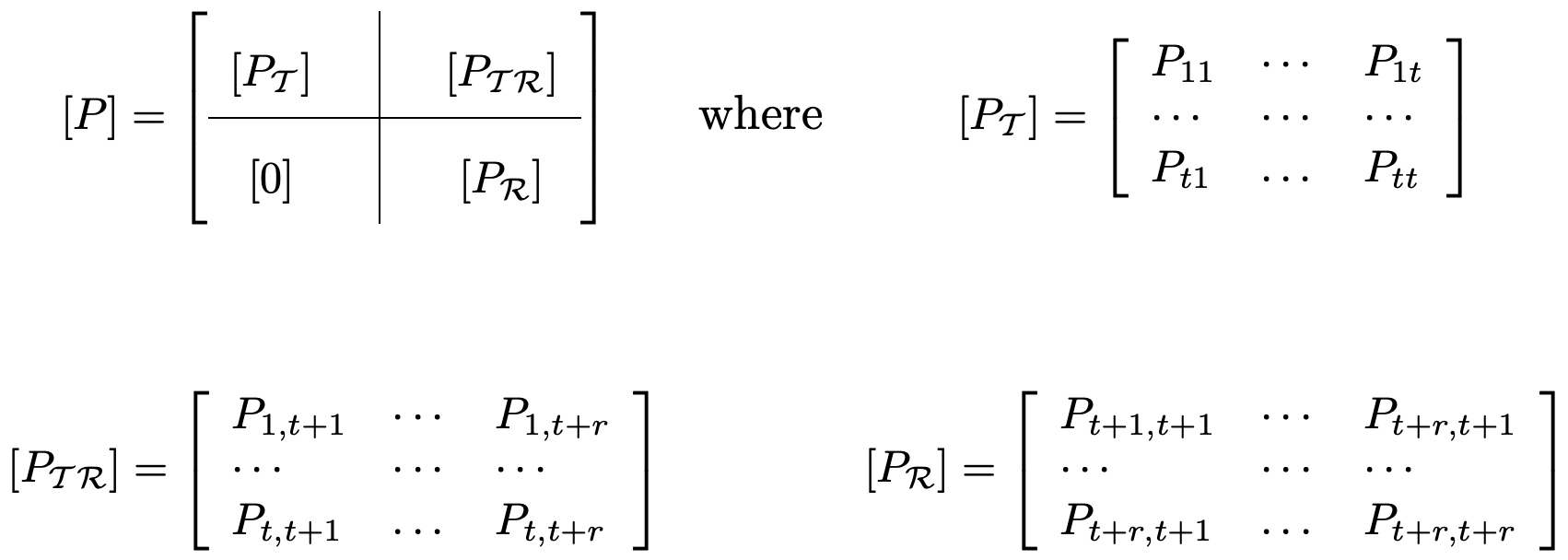Figure 3.5: The transition matrix of a unichain. The block of zeroes in the lower left corresponds to the absence of transitions from recurrent to transient states.

assume the states of \(\mathcal{T}\) are numbered 1, 2, . . . , \(t\). Let \(\mathcal{R}\) denote the recurrent class, assumed to be numbered \(t+1, \ldots, t+r\) (see Figure 3.5).

If \(i\) and \(j\) are both recurrent states, then there is no possibility of leaving the recurrent class in going from \(i\) to \(j\). Assuming this class to be ergodic, the transition matrix \(\left[P_{\mathcal{R}}\right]\) as shown in Figure 3.5 has been analyzed in Section 3.3.3.

If the initial state is a transient state, then eventually the recurrent class is entered, and eventually after that, the distribution approaches steady state within the recurrent class. This suggests (and we next show) that there is a steady-state vector \(\boldsymbol{\pi}\) for \([P]\) itself such that \(\pi_{j}=0\) for \(j \in \mathcal{T}\) and \(\pi j\) is as given in Section 3.3.3 for each \(j \in \mathcal{R}\).

Initially we will show that \(P_{i j}^{n}\) converges to 0 for \(i, j \in \mathcal{T}\). The exact nature of how and ij when the recurrent class is entered starting in a transient state is an interesting problem in its own right, and is discussed more later. For now, a crude bound will suffice.

For each transient state, there must a walk to some recurrent state, and since there are only \(t\) transient states, there must be some such path of length at most \(t\). Each such path has positive probability, and thus for each \(i \in \mathcal{T}\), \(\sum_{j \in \mathcal{R}} P_{i j}^{t}>0\). It follows that for each \(i \in \mathcal{T}\), \(\sum_{j \in \mathcal{T}} P_{i j}^{t}<1\). Let \(\gamma<1\) be the maximum of these probabilities over \(i \in \mathcal{T}\), i.e.,

\(\gamma=\max _{i \in \mathcal{T}} \sum_{j \in \mathcal{T}} P_{i j}^{t}<1\)

Theorem 3.3.3

Let \([P]\) be a unichain with a set \(\mathcal{T}\) of \(t\) transient states. Then

\[\max _{\ell \in \mathcal{T}} \sum_{j \in \mathcal{T}} P_{\ell j}^{n} \leq \gamma^{\lfloor n / t\rfloor}\label{3.24} \]

Proof

For each integer multiple \(\nu t\) and each \(i \in \mathcal{T}\),

\(\sum_{j \in \mathcal{T}} P_{i j}^{(\nu+1) t}=\sum_{k \in \mathcal{T}} P_{i k}^{t} \sum_{j \in \mathcal{T}} P_{k j}^{\nu t} \leq \sum_{k \in \mathcal{T}} P_{i k}^{t} \max _{\ell \in \mathcal{T}} \sum_{j \in \mathcal{T}} P_{\ell j}^{\nu t} \leq \gamma \max _{\ell \in \mathcal{T}} \sum_{j \in \mathcal{T}} P_{\ell j}^{\nu t}\)

Recognizing that this applies to all \(i \in \mathcal{T}\), and thus to the maximum over \(i\), we can iterate this equation, getting

\(\max _{\ell \in \mathcal{T}} \sum_{j \in \mathcal{T}} P_{\ell j}^{\nu t} \leq \gamma^{\nu}\)

Since this maximum is nonincreasing in \(n\), \ref{3.24} follows.

We now proceed to the case where the initial state is \(i \in \mathcal{T}\) and the final state is \(j \in \mathcal{R}\). Let \(m=\lfloor n / 2\rfloor\). For each \(i \in \mathcal{T}\) and \(j \in \mathcal{R}\), the Chapman-Kolmogorov equation, says that

\(P_{i j}^{n}=\sum_{k \in \mathcal{T}} P_{i k}^{m} P_{k j}^{n-m}+\sum_{k \in \mathcal{R}} P_{i k}^{m} P_{k j}^{n-m}\)

Let \(\pi j\) be the steady-state probability of state \(j \in \mathcal{R}\) in the recurrent Markov chain with states \(\mathcal{R}\), i.e., \(\pi_{j}=\lim _{n \rightarrow \infty} P_{k j}^{n}\). Then for each \(i \in \mathcal{T}\),

\(\begin{aligned}
\left|P_{i j}^{n}-\pi_{j}\right| &=\left|\sum_{k \in \mathcal{T}} P_{i k}^{m}\left(P_{k j}^{n-m}-\pi_{j}\right)+\sum_{k \in \mathcal{R}} P_{i k}^{m}\left(P_{k j}^{n-m}-\pi_{j}\right)\right| \\
& \leq \sum_{k \in \mathcal{T}} P_{i k}^{m}\left|P_{k j}^{n-m}-\pi_{j}\right|+\sum_{k \in \mathcal{R}} P_{i k}^{m}\left|P_{k j}^{n-m}-\pi_{j}\right| \\
& \leq \sum_{k \in \mathcal{T}} P_{i k}^{m}+\sum_{k \in \mathcal{R}} P_{i k}^{m}\left|P_{k j}^{n-m}-\pi_{j}\right| \quad&(3.25)\\
& \leq \gamma^{\lfloor m / t\rfloor}+(1-2 \beta)^{\lfloor(n-m) / h\rfloor},&\quad(3.26)
\end{aligned}\)

where the first step upper bounded the absolute value of a sum by the sum of the absolute values. In the last step, \ref{3.24} was used in the first half of \ref{3.25} and \ref{3.21} (with \(h=(r-1)^{2}-1\) and \(\beta=\min _{i, j \in \mathcal{R}} P_{i j}^{h}>0\) was used in the second half.

This is summarized in the following theorem.

Theorem 3.3.2

Let \([P]\) be the matrix of an ergodic finite-state unichain. Then \(\lim _{n \rightarrow \infty}\left[P^{n}\right]=\boldsymbol{e\pi}\) where \(\boldsymbol{e}=(1,1, \ldots, 1)^{T}\) and \(\boldsymbol{\pi}\) is the steady-state vector of the recurrent class of states, expanded by 0’s for each transient state of the unichain. The convergence is exponential in \(n\) for all \(i\), \(j\).

Arbitrary finite-state Markov chains

The asymptotic behavior of \(\left[P^{n}\right]\) as \(n \rightarrow \infty\) for arbitrary finite-state Markov chains can mostly be deduced from the ergodic unichain case by simple extensions and common sense.

First consider the case of \(m>1\) aperiodic classes plus a set of transient states. If the initial state is in the ∑th of the recurrent classes, say \(\mathcal{R}^{\kappa}\) then the chain remains in \(\mathcal{R}^{\kappa}\) and there is a unique finite-state vector \(\boldsymbol{\pi}^{\kappa}\) that is non-zero only in \(\mathcal{R}^{\kappa}\) that can be found by viewing class \(\kappa\) in isolation.

If the initial state i is transient, then, for each \(\mathcal{R}^{\kappa}\), there is a certain probability that \(\mathcal{R}^{\kappa}\) is eventually reached, and once it is reached there is no exit, so the steady state over that recurrent class is approached. The question of finding the probability of entering each recurrent class from a given transient class will be discussed in the next section.

Next consider a recurrent Markov chain that is periodic with period \(d\). The \(d\)th order transition probability matrix, \(\left[P^{d}\right]\), is then constrained by the fact that \(P_{i j}^{d}=0\) for all \(j\) not in the same periodic subset as \(i\). In other words, \(\left[P^{d}\right]\) is the matrix of a chain with \(d\) recurrent classes. We will obtain greater facility in working with this in the next section when eigenvalues and eigenvectors are discussed.

---

Reference

⁴One might naively try to show that a steady-state vector exists by first noting that each row of \(P\) sums to 1. The column vector \(\boldsymbol{e}=(1,1, \ldots, 1)^{\top}\) then satisfies the eigenvector equation \(\boldsymbol{e}=[P] \boldsymbol{e}\). Thus there must also be a left eigenvector satisfying \(\boldsymbol{\pi}[P]=\boldsymbol{\pi}\). The problem here is showing that \(\boldsymbol{\pi}\) is real and non-negative.

⁵This is essentially the Frobenius theorem for non-negative irreducible matrices, specialized to Markov chains. A non-negative matrix \([P]\) is irreducible if its graph (containing an edge from node \(i\) to \(j\) if \(P_{i j}>0\)) is the graph of a recurrent Markov chain. There is no constraint that each row of \([P]\) sums to 1. The proof of the Frobenius theorem requires some fairly intricate analysis and seems to be far more complex than the simple proof here for Markov chains. A proof of the general Frobenius theorem can be found in [10].