3.5: Markov Chains with Rewards

Suppose that each state in a Markov chain is associated with a reward, \(r_{i}\). As the Markov chain proceeds from state to state, there is an associated sequence of rewards that are not independent, but are related by the statistics of the Markov chain. The concept of a reward in each state¹¹ is quite graphic for modeling corporate profits or portfolio performance, and is also useful for studying queueing delay, the time until some given state is entered, and many other phenomena. The reward \(r_{i}\) associated with a state could equally well be viewed as a cost or any given real-valued function of the state.

In Section 3.6, we study dynamic programming and Markov decision theory. These topics include a “decision maker,” “policy maker,” or “control” that modify both the transition probabilities and the rewards at each trial of the ‘Markov chain.’ The decision maker attempts to maximize the expected reward, but is typically faced with compromising between immediate reward and the longer-term reward arising from the choice of transition probabilities that lead to ‘high reward’ states. This is a much more challenging problem than the current study of Markov chains with rewards, but a thorough understanding of the current problem provides the machinery to understand Markov decision theory also.

The steady-state expected reward per unit time, assuming a single recurrent class of states, is defined to be the gain, expressed as \(g=\sum_{i} \pi_{i} r_{i}\) where \(\pi_{i}\) is the steady-state probability

Examples of Markov Chains with Rewards

The following examples demonstrate that it is important to understand the transient behavior of rewards as well as the long-term averages. This transient behavior will turn out to be even more important when we study Markov decision theory and dynamic programming.

Example 3.5.1: Expected first-passage time

First-passage times, i.e., the number of steps taken in going from one given state, say \(i\), to another, say 1, are frequently of interest for Markov chains, and here we solve for the expected value of this random variable.

Solution

Since the first-passage time is independent of the transitions after the first entry to state 1, we can modify the chain to convert the final state, say state 1, into a trapping state (a trapping state \(i\) is a state from which there is no exit, i.e., for which \(P_{i i}=1\)). That is, we modify \(P_{11}\) to 1 and \(P_{1 j}\) to 0 for all \(j \neq 1\). We leave \(P_{i j}\) unchanged for all \(i \neq 1\) and all \(j\) (see Figure 3.6). This modification of the chain will not change the probability of any sequence of states up to the point that state 1 is first entered.

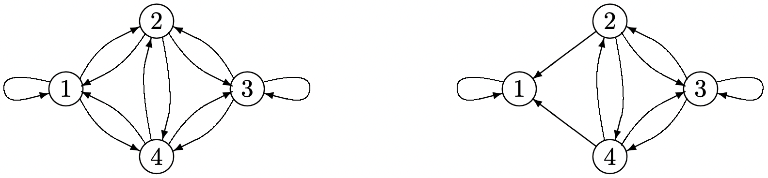Figure 3.6: The conversion of a recurrent Markov chain with M = 4 into a chain for which state 1 is a trapping state, i.e., the outgoing arcs from node 1 have been removed.

Let \(v_{i}\) be the expected number of steps to first reach state 1 starting in state \(i \neq 1\). This number of steps includes the first step plus the expected number of remaining steps to reach state 1 starting from whatever state is entered next (if state 1 is the next state entered, this remaining number is 0). Thus, for the chain in Figure 3.6, we have the equations

\(\begin{aligned}
v_{2} &=1+P_{23} v_{3}+P_{24} v_{4} \\
v_{3} &=1+P_{32} v_{2}+P_{33} v_{3}+P_{34} v_{4} \\
v_{4} &=1+P_{42} v_{2}+P_{43} v_{3}
\end{aligned}\)

For an arbitrary chain of M states where 1 is a trapping state and all other states are transient, this set of equations becomes

\[v_{i}=1+\sum_{j \neq 1} P_{i j} v_{j} ; \quad i \neq 1\label{3.31} \]

If we define \(r_{i}=1\) for \(i \neq 1\) and \(r_{i}=0\) for \(i=1\), then \(r_{i}\) is a unit reward for not yet entering the trapping state, and \(v_{i}\) is the expected aggregate reward before entering the trapping state. Thus by taking \(r_{1}=0\), the reward ceases upon entering the trapping state, and \(v_{i}\) is the expected transient reward, i.e., the expected first-passage time from state \(i\) to state 1. Note that in this example, rewards occur only in transient states. Since transient states have zero steady-state probabilities, the steady-state gain per unit time, \(g=\sum_{i} \pi_{i} r_{i}\), is 0.

If we define \(v_{1}=0\), then (3.31), along with \(v_{1}=0\), has the vector form

\[\boldsymbol{v}=\boldsymbol{r}+[P] \boldsymbol{v} ; \quad v_{1}=0\label{3.32} \]

For a Markov chain with M states, \ref{3.31} is a set of M − 1 equations in the M − 1 variables \(v_{2}\) to \(v_{M}\). The equation \(\boldsymbol{v}=\boldsymbol{r}+[P] \boldsymbol{v}\) is a set of M linear equations, of which the first is the vacuous equation \(v_{1}=0+v_{1}\), and, with \(v_{1}=0\), the last M − 1 correspond to (3.31). It is not hard to show that \ref{3.32} has a unique solution for \(\boldsymbol{v}\) under the condition that states 2 to M are all transient and 1 is a trapping state, but we prove this later, in Theorem 3.5.1, under more general circumstances.

Example 3.5.2

Assume that a Markov chain has M states, \(\{0,1, \ldots, \mathrm{M}-1\}\), and that the state represents the number of customers in an integer-time queueing system. Suppose we wish to find the expected sum of the customer waiting times, starting with \(i\) customers in the system at some given time \(t\) and ending at the first instant when the system becomes idle. That is, for each of the \(i\) customers in the system at time \(t\), the waiting time is counted from \(t\) until that customer exits the system. For each new customer entering before the system next becomes idle, the waiting time is counted from entry to exit.

Solution

When we discuss Little’s theorem in Section 4.5.4, it will be seen that this sum of waiting times is equal to the sum over \(\tau\) of the state \(X_{\tau}\) at time \(\tau\), taken from \(\tau=t\) to the first subsequent time the system is empty.

As in the previous example, we modify the Markov chain to make state 0 a trapping state and assume the other states are then all transient. We take \(r_{i}=i\) as the “reward” in state \(i\), and \(v_{i}\) as the expected aggregate reward until the trapping state is entered. Using the same reasoning as in the previous example, \(v_{i}\) is equal to the immediate reward \(r_{i}=i\) plus the expected aggregate reward from whatever state is entered next. Thus \(v_{i}=r_{i}+\sum_{j \geq 1} P_{i j} v_{j}\). With \(v_{0}=0\), this is \(\boldsymbol{v}=\boldsymbol{r}+[P] \boldsymbol{v}\). This has a unique solution for \(\boldsymbol{v}\), as will be shown later in Theorem 3.5.1. This same analysis is valid for any choice of reward \(r_{i}\) for each transient state \(i\); the reward in the trapping state must be 0 so as to keep the expected aggregate reward finite.

In the above examples, the Markov chain is converted into a trapping state with zero gain, and thus the expected reward is a transient phenomena with no reward after entering the trapping state. We now look at the more general case of a unichain. In this more general case, there can be some gain per unit time, along with some transient expected reward depending on the initial state. We first look at the aggregate gain over a finite number of time units, thus providing a clean way of going to the limit.

Example 3.5.3

The example in Figure 3.7 provides some intuitive appreciation for the general problem. Note that the chain tends to persist in whatever state it is in. Thus if the chain starts in state 2, not only is an immediate reward of 1 achieved, but there is a high probability of additional unit rewards on many successive transitions. Thus the aggregate value of starting in state 2 is considerably more than the immediate reward of 1. On the other hand, we see from symmetry that the gain per unit time, over a long time period, must be one half.

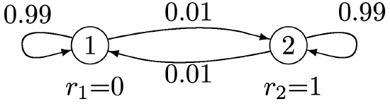Figure 3.7: Markov chain with rewards and nonzero steady-state gain.

Expected Aggregate Reward over Multiple Transitions

Returning to the general case, let \(X_{m}\) be the state at time \(m\) and let \(R_{m}=R\left(X_{m}\right)\) be the reward at that \(m\), i.e., if the sample value of \(X_{m}\) is \(i\), then \(r_{i}\) is the sample value of \(R_{m}\). Conditional on \(X_{m}=i\), the aggregate expected reward \(v_{i}(n)\) over \(n\) trials from \(X_{m}\) to \(X_{m+n-1}\) is

\(\begin{aligned}
v_{i}(n) &=\mathrm{E}\left[R\left(X_{m}\right)+R\left(X_{m+1}\right)+\cdots+R\left(X_{m+n-1}\right) \mid X_{m}=i\right] \\
&=r_{i}+\sum_{j} P_{i j} r_{j}+\cdots+\sum_{j} P_{i j}^{n-1} r_{j}
\end{aligned}\)

This expression does not depend on the starting time \(m\) because of the homogeneity of the Markov chain. Since it gives the expected reward for each initial state \(i\), it can be combined into the following vector expression \(\boldsymbol{v}(n)=\left(v_{1}(n), v_{2}(n), \ldots, v_{\mathrm{M}}(n)\right)^{\top}\),

\[\boldsymbol{v}(n)=\boldsymbol{r}+[P] \boldsymbol{r}+\cdots+\left[P^{n-1}\right] \boldsymbol{r}=\sum_{h=0}^{n-1}\left[P^{h}\right] \boldsymbol{r}\label{3.33} \]

where \(\boldsymbol{r}=\left(r_{1}, \ldots, r_{\mathrm{M}}\right)^{\top}\) and \(P^{0}\) is the identity matrix. Now assume that the Markov chain is an ergodic unichain. Then \(\lim _{n \rightarrow \infty}[P]^{n}=\boldsymbol{e} \boldsymbol{\pi}\) and \(\lim _{n \rightarrow \infty}[P]^{n} \boldsymbol{r}=\boldsymbol{e} \boldsymbol{\pi} \boldsymbol{r}=g \boldsymbol{e}\) where \(g=\boldsymbol{\pi r}\) is the steady-state reward per unit time. If \(g \neq 0\), then \(\boldsymbol{v}(n)\) changes by approximately \(g \boldsymbol{e}\) for each unit increase in \(n\), so \(\boldsymbol{v}(n)\) does not have a limit as \(n \rightarrow \infty\). As shown below, however, \(\boldsymbol{v}(n)-n g \boldsymbol{e}\) does have a limit, given by

\[\lim _{n \rightarrow \infty}(\boldsymbol{v}(n)-n g \boldsymbol{e})=\lim _{n \rightarrow \infty} \sum_{h=0}^{n-1}\left[P^{h}-\boldsymbol{e} \boldsymbol{\pi}\right] \boldsymbol{r}\label{3.34} \]

To see that this limit exists, note from \ref{3.26} that \(\epsilon>0\) can be chosen small enough that \(P_{i j}^{n}-\pi_{j}=o(\exp (-n \epsilon))\) for all states \(i\), \(j\) and all \(n \geq 1\). Thus \(\sum_{h=n}^{\infty}\left(P_{i j}^{h}-\pi_{j}\right)=o(\exp (-n \epsilon))\) also. This shows that the limits on each side of \ref{3.34} must exist for an ergodic unichain.

The limit in \ref{3.34} is a vector over the states of the Markov chain. This vector gives the asymptotic relative expected advantage of starting the chain in one state relative to another. This is an important quantity in both the next section and the remainder of this one. It is called the relative-gain vector and denoted by \(\boldsymbol{w}\),

\[\begin{aligned}
\boldsymbol{w} &=\lim _{n \rightarrow \infty} \sum_{h=0}^{n-1}\left[P^{h}-\boldsymbol{e} \boldsymbol{\pi}\right] \boldsymbol{r}&(3.35) \\
&=\lim _{n \rightarrow \infty}(\boldsymbol{v}(n)-n g \boldsymbol{e}) .&(3.36)
\end{aligned} \nonumber \]

Note from \ref{3.36} that if \(g>0\), then \(ng\boldsymbol{e}\) increases linearly with \(n\) and and \(\boldsymbol{v}(n)\) must asymptotically increase linearly with \(n\). Thus the relative-gain vector \(\boldsymbol{w}\) becomes small relative to both \(ng\boldsymbol{e}\) and \(\boldsymbol{v}(n)\) for large \(n\). As we will see, \(\boldsymbol{w}\) is still important, particularly in the next section on Markov decisions.

We can get some feel for \(\boldsymbol{w}\) and how \(v_{i}(n)-n \pi_{i}\) converges to \(w_{i}\) from Example 3.5.3 (as described in Figure 3.7). Since this chain has only two states, \(\left[P^{n}\right]\) and \(v_{i}(n)\) can be calculated easily from (3.28). The result is tabulated in Figure 3.8, and it is seen numerically that \(\boldsymbol{w}=(-25,+25)^{\top}\). The rather significant advantage of starting in state 2 rather than 1, however, requires hundreds of transitions before the gain is fully apparent.

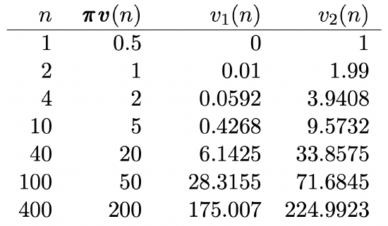Figure 3.8: The expected aggregate reward, as a function of starting state and stage, for the example of figure 3.7. Note that \(\boldsymbol{w}=(-25,+25)^{\top}\), but the convergence is quite slow.

This example also shows that it is somewhat inconvenient to calculate \(\boldsymbol{w}\) from (3.35), and this inconvenience grows rapidly with the number of states. Fortunately, as shown in the following theorem, \(\boldsymbol{w}\) can also be calculated simply by solving a set of linear equations.

Theorem 3.5.1

Let \([P]\) be the transition matrix for an ergodic unichain. Then the relativegain vector \(\boldsymbol{w}\) given in \ref{3.35} satisfies the following linear vector equation.

\[\boldsymbol{w}+g \boldsymbol{e}=[P] \boldsymbol{w}+\boldsymbol{r} \quad \text { and } \boldsymbol{\pi} \boldsymbol{w}=0\label{3.37} \]

Furthermore \ref{3.37} has a unique solution if \([P]\) is the transition matrix for a unichain (either ergodic or periodic).

Discussion

For an ergodic unichain, the interpretation of \(\boldsymbol{w}\) as an asymptotic relative gain comes from \ref{3.35} and (3.36). For a periodic unichain, \ref{3.37} still has a unique solution, but \ref{3.35} no longer converges, so the solution to \ref{3.37} no longer has a clean interpretation as an asymptotic limit of relative gain. This solution is still called a relative-gain vector, and can be interpreted as an asymptotic relative gain over a period, but the important thing is that this equation has a unique solution for arbitrary unichains

Definition 3.5.1

The relative-gain vector \(\boldsymbol{w}\) of a unichain is the unique vector that satisfies (3.37).

Proof

Premultiplying both sides of \ref{3.35} by \([P]\),

\(\begin{aligned}{}
[P] \boldsymbol{w} &=\lim _{n \rightarrow \infty} \sum_{h=0}^{n-1}\left[P^{h+1}-\boldsymbol{e} \boldsymbol{\pi}\right] \boldsymbol{r} \\
&=\lim _{n \rightarrow \infty} \sum_{h=1}^{n}\left[P^{h}-\boldsymbol{e} \boldsymbol{\pi}\right] \boldsymbol{r} \\
&=\lim _{n \rightarrow \infty}\left(\sum_{h=0}^{n}\left[P^{h}-\boldsymbol{e} \boldsymbol{\pi}\right] \boldsymbol{r}\right)-\left[P^{0}-\boldsymbol{e} \boldsymbol{\pi}\right] \boldsymbol{r} \\
&=\boldsymbol{w}-\left[P^{0}\right] \boldsymbol{r}+\boldsymbol{e} \boldsymbol{\pi} \boldsymbol{r}=\boldsymbol{w}-\boldsymbol{r}+g \boldsymbol{e}
\end{aligned}\)

Rearranging terms, we get (3.37). For a unichain, the eigenvalue 1 of \([P]\) has multiplicity 1, and the existence and uniqueness of the solution to \ref{3.37} is then a simple result in linear algebra (see Exercise 3.23).

The above manipulations conceal the intuitive nature of (3.37). To see the intuition, consider the first-passage-time example again. Since all states are transient except state 1, \(\pi_{1}=1\). Since \(r_{1}=0\), we see that the steady-state gain is \(g=0\). Also, in the more general model of the theorem, \(v_{i}(n)\) is the expected reward over \(n\) transitions starting in state \(i\), which for the first-passage-time example is the expected number of transient states visited up to the \(n\)th transition. In other words, the quantity \(v_{i}\) in the first-passage-time example is \(\lim _{n \rightarrow \infty} v_{i}(n)\). This means that the \(\boldsymbol{v}\) in \ref{3.32} is the same as \(\boldsymbol{w}\) here, and it is seen that the formulas are the same with \(g\) set to 0 in (3.37).

The reason that the derivation of aggregate reward was so simple for first-passage time is that there was no steady-state gain in that example, and thus no need to separate the gain per transition \(g\) from the relative gain \(\boldsymbol{w}\) between starting states.

One way to apply the intuition of the \(g=0\) case to the general case is as follows: given a reward vector \(\boldsymbol{r}\), find the steady-state gain \(g=\boldsymbol{\pi} \boldsymbol{r}\), and then define a modified reward vector \(\boldsymbol{r}^{\prime}=\boldsymbol{r}-g \boldsymbol{e}\). Changing the reward vector from \(\boldsymbol{r}\) to \(\boldsymbol{r}^{\prime}\) in this way does not change \(\boldsymbol{w}\), but the modified limiting aggregate gain, say \(\boldsymbol{v}^{\prime}(n)\) then has a limit, which is in fact \(\boldsymbol{w}\). The intuitive derivation used in \ref{3.32} again gives us \(\boldsymbol{w}=[P] \boldsymbol{w}+{\boldsymbol{r}}^{\prime}\). This is equivalent to \ref{3.37} since \(\boldsymbol{r}^{\prime}=\boldsymbol{r}-g \boldsymbol{e}\).

There are many generalizations of the first-passage-time example in which the reward in each recurrent state of a unichain is 0. Thus reward is accumulated only until a recurrent state is entered. The following corollary provides a monotonicity result about the relativegain vector for these circumstances that might seem obvious¹². Thus we simply state it and give a guided proof in Exercise 3.25.

Corollary 3.5.1

Let \([P]\) be the transition matrix of a unichain with the recurrent class \(\mathcal{R}\). Let \(\boldsymbol{r} \geq 0\) be a reward vector for \([P]\) with \(r_{i}=0\) for \(i \in \mathcal{R}\). Then the relative-gain vector \(\boldsymbol{w}\) satisfies \(\boldsymbol{w} \geq 0\) with \(w_{i}=0\) for \(i \in \mathcal{R}\) and \(w_{i}>0\) for \(r_{i}>0\). Furthermore, if \(\boldsymbol{r}^{\prime}\) and \(\boldsymbol{r}^{\prime \prime}\) are different reward vectors for \([P]\) and \(\boldsymbol{r}^{\prime} \geq \boldsymbol{r}^{\prime \prime}\) with \(r_{i}^{\prime}=r_{i}^{\prime \prime}\) for \(i \in \mathcal{R}\), then \(\boldsymbol{w}^{\prime} \geq \boldsymbol{w}^{\prime \prime}\) with \(w_{i}^{\prime}=w_{i}^{\prime \prime}\) for \(i \in \mathcal{R}\) and \(w_{i}^{\prime}>w_{i}^{\prime \prime}\) for \(r_{i}^{\prime}>r_{i}^{\prime \prime}\).

Expected Aggregate Reward with an Additional Final Reward

Frequently when a reward is aggregated over \(n\) transitions of a Markov chain, it is appropriate to assign some added reward, say \(u_{i}\), as a function of the final state \(i\). For example, it might be particularly advantageous to end in some particular state. Also, if we wish to view the aggregate reward over \(n+\ell\) transitions as the reward over the first \(n\) transitions plus that over the following \(\ell\) transitions, we can model the expected reward over the final \(\ell\) transitions as a final reward at the end of the first \(n\) transitions. Note that this final expected reward depends only on the state at the end of the first \(n\) transitions.

As before, let \(R\left(X_{m+h}\right)\) be the reward at time \(m+h\) for \(0 \leq h \leq n-1\) and \(U\left(X_{m+n}\right)\) be the final reward at time \(m+n\), where \(U(X)=u_{i}\) for \(X=i\). Let \(v_{i}(n, \boldsymbol{u})\) be the expected reward from time \(m\) to \(m+n\), using the reward \(\boldsymbol{r}\) from time \(m\) to \(m+n-1\) and using the final reward \(\boldsymbol{u}\) at time \(m+n\). The expected reward is then the following simple modification of (3.33):

\[\boldsymbol{v}(n, \boldsymbol{u})=\boldsymbol{r}+[P] \boldsymbol{r}+\cdots+\left[P^{n-1}\right] \boldsymbol{r}+\left[P^{n}\right] \boldsymbol{u}=\sum_{h=0}^{n-1}\left[P^{h}\right] \boldsymbol{r}+\left[P^{n}\right] \boldsymbol{u}\label{3.38} \]

This simplifies considerably if \(\boldsymbol{u}\) is taken to be the relative-gain vector \(\boldsymbol{w}\).

Theorem 3.5.2

Let \([P]\) be the transition matrix of a unichain and let \(\boldsymbol{w}\) be the corresponding relative-gain vector. Then for each \(n \geq 1\),

\[\boldsymbol{v}(n, \boldsymbol{w})=n g \boldsymbol{e}+\boldsymbol{w}\label{3.39} \]

Also, for an arbitrary final reward vector \(\boldsymbol{u}\),

\[\boldsymbol{v}(n, \boldsymbol{u})=n g \boldsymbol{e}+\boldsymbol{w}+\left[P^{n}\right](\boldsymbol{u}-\boldsymbol{w})\label{3.40} \]

Discussion

An important special case of \ref{3.40} arises from setting the final reward \(\boldsymbol{u}\) to 0, thus yielding the following expression for \(\boldsymbol{v}(n)\):

\[\boldsymbol{v}(n)=n g \boldsymbol{e}+\boldsymbol{w}-\left[P^{n}\right] \boldsymbol{w}\label{3.41} \]

For an ergodic unichain, \(\lim _{n \rightarrow \infty}\left[P^{n}\right]=\boldsymbol{e} \boldsymbol{\pi}\). Since \(\boldsymbol{\pi} \boldsymbol{w}=0\) by definition of \(\boldsymbol{w}\), the limit of \ref{3.41} as \(n \rightarrow \infty\) is

\(\lim _{n \rightarrow \infty}(\boldsymbol{v}(n)-n g \boldsymbol{e})=\boldsymbol{w},\)

which agrees with (3.36). The advantage of \ref{3.41} over \ref{3.36} is that it provides an explicit expression for \(\boldsymbol{v}(n)\) for each \(n\) and also that it continues to hold for a periodic unichain.

Proof

For \(n=1\), we see from \ref{3.38} that

\(\boldsymbol{v}(1, \boldsymbol{w})=\boldsymbol{r}+[P] \boldsymbol{w}=g \boldsymbol{e}+\boldsymbol{w},\)

so the theorem is satisfied for \(n = 1\). For \(n>1\),

\(\begin{aligned}
\boldsymbol{v}(n, \boldsymbol{w}) &=\sum_{h=0}^{n-1}\left[P^{h}\right] \boldsymbol{r}+\left[P^{n}\right] \boldsymbol{w} \\
&=\sum_{h=0}^{n-2}\left[P^{h}\right] \boldsymbol{r}+\left[P^{n-1}\right](\boldsymbol{r}+[P] \boldsymbol{w}) \\
&=\sum_{h=0}^{n-2}\left[P^{h}\right] \boldsymbol{r}+\left[P^{n-1}\right](g \boldsymbol{e}+\boldsymbol{w}) \\
&=\boldsymbol{v}(n-1, \boldsymbol{w})+g \boldsymbol{e} .
\end{aligned}\)

Using induction, this implies (3.39).

To establish (3.40), note from \ref{3.38} that

\(\boldsymbol{v}(n, \boldsymbol{u})-\boldsymbol{v}(n, \boldsymbol{w})=\left[P^{n}\right](\boldsymbol{u}-\boldsymbol{w})\)

Then \ref{3.40} follows by using \ref{3.39} for the value of \(\boldsymbol{v}(n, \boldsymbol{w})\)

---

Reference

⁹See Strang [19], for example, for a more complete description of how to construct a Jordan form

¹⁰This polynomial is equal to 1 if these eigenvalues are simple.

¹¹Occasionally it is more natural to associate rewards with transitions rather than states. If \(r_{i j}\) denotes a reward associated with a transition from \(i\) to \(j\) and \(P_{i j}\) denotes the corresponding transition probability, then defining \(r_{i}=\sum_{j} P_{i j} r_{i j}\) essentially simplifies these transition rewards to rewards over the initial state for the transition. These transition rewards are ignored here, since the details add complexity to a topic that is complex enough for a first treatment.

¹²An obvious counterexample if we omit the condition \(r_{i}=0\) for \(i \in \mathcal{R}\) is given by Figure 3.7 where \(\boldsymbol{r}=(0,1)^{\top}\) and \(\boldsymbol{w}=(-25,25)^{\top}\).