
3.6: Markov Decision Theory and Dynamic Programming
- Page ID
- 75817
\( \newcommand{\vecs}[1]{\overset { \scriptstyle \rightharpoonup} {\mathbf{#1}} } \)
\( \newcommand{\vecd}[1]{\overset{-\!-\!\rightharpoonup}{\vphantom{a}\smash {#1}}} \)
\( \newcommand{\dsum}{\displaystyle\sum\limits} \)
\( \newcommand{\dint}{\displaystyle\int\limits} \)
\( \newcommand{\dlim}{\displaystyle\lim\limits} \)
\( \newcommand{\id}{\mathrm{id}}\) \( \newcommand{\Span}{\mathrm{span}}\)
( \newcommand{\kernel}{\mathrm{null}\,}\) \( \newcommand{\range}{\mathrm{range}\,}\)
\( \newcommand{\RealPart}{\mathrm{Re}}\) \( \newcommand{\ImaginaryPart}{\mathrm{Im}}\)
\( \newcommand{\Argument}{\mathrm{Arg}}\) \( \newcommand{\norm}[1]{\| #1 \|}\)
\( \newcommand{\inner}[2]{\langle #1, #2 \rangle}\)
\( \newcommand{\Span}{\mathrm{span}}\)
\( \newcommand{\id}{\mathrm{id}}\)
\( \newcommand{\Span}{\mathrm{span}}\)
\( \newcommand{\kernel}{\mathrm{null}\,}\)
\( \newcommand{\range}{\mathrm{range}\,}\)
\( \newcommand{\RealPart}{\mathrm{Re}}\)
\( \newcommand{\ImaginaryPart}{\mathrm{Im}}\)
\( \newcommand{\Argument}{\mathrm{Arg}}\)
\( \newcommand{\norm}[1]{\| #1 \|}\)
\( \newcommand{\inner}[2]{\langle #1, #2 \rangle}\)
\( \newcommand{\Span}{\mathrm{span}}\) \( \newcommand{\AA}{\unicode[.8,0]{x212B}}\)
\( \newcommand{\vectorA}[1]{\vec{#1}} % arrow\)
\( \newcommand{\vectorAt}[1]{\vec{\text{#1}}} % arrow\)
\( \newcommand{\vectorB}[1]{\overset { \scriptstyle \rightharpoonup} {\mathbf{#1}} } \)
\( \newcommand{\vectorC}[1]{\textbf{#1}} \)
\( \newcommand{\vectorD}[1]{\overrightarrow{#1}} \)
\( \newcommand{\vectorDt}[1]{\overrightarrow{\text{#1}}} \)
\( \newcommand{\vectE}[1]{\overset{-\!-\!\rightharpoonup}{\vphantom{a}\smash{\mathbf {#1}}}} \)
\( \newcommand{\vecs}[1]{\overset { \scriptstyle \rightharpoonup} {\mathbf{#1}} } \)
\(\newcommand{\longvect}{\overrightarrow}\)
\( \newcommand{\vecd}[1]{\overset{-\!-\!\rightharpoonup}{\vphantom{a}\smash {#1}}} \)
\(\newcommand{\avec}{\mathbf a}\) \(\newcommand{\bvec}{\mathbf b}\) \(\newcommand{\cvec}{\mathbf c}\) \(\newcommand{\dvec}{\mathbf d}\) \(\newcommand{\dtil}{\widetilde{\mathbf d}}\) \(\newcommand{\evec}{\mathbf e}\) \(\newcommand{\fvec}{\mathbf f}\) \(\newcommand{\nvec}{\mathbf n}\) \(\newcommand{\pvec}{\mathbf p}\) \(\newcommand{\qvec}{\mathbf q}\) \(\newcommand{\svec}{\mathbf s}\) \(\newcommand{\tvec}{\mathbf t}\) \(\newcommand{\uvec}{\mathbf u}\) \(\newcommand{\vvec}{\mathbf v}\) \(\newcommand{\wvec}{\mathbf w}\) \(\newcommand{\xvec}{\mathbf x}\) \(\newcommand{\yvec}{\mathbf y}\) \(\newcommand{\zvec}{\mathbf z}\) \(\newcommand{\rvec}{\mathbf r}\) \(\newcommand{\mvec}{\mathbf m}\) \(\newcommand{\zerovec}{\mathbf 0}\) \(\newcommand{\onevec}{\mathbf 1}\) \(\newcommand{\real}{\mathbb R}\) \(\newcommand{\twovec}[2]{\left[\begin{array}{r}#1 \\ #2 \end{array}\right]}\) \(\newcommand{\ctwovec}[2]{\left[\begin{array}{c}#1 \\ #2 \end{array}\right]}\) \(\newcommand{\threevec}[3]{\left[\begin{array}{r}#1 \\ #2 \\ #3 \end{array}\right]}\) \(\newcommand{\cthreevec}[3]{\left[\begin{array}{c}#1 \\ #2 \\ #3 \end{array}\right]}\) \(\newcommand{\fourvec}[4]{\left[\begin{array}{r}#1 \\ #2 \\ #3 \\ #4 \end{array}\right]}\) \(\newcommand{\cfourvec}[4]{\left[\begin{array}{c}#1 \\ #2 \\ #3 \\ #4 \end{array}\right]}\) \(\newcommand{\fivevec}[5]{\left[\begin{array}{r}#1 \\ #2 \\ #3 \\ #4 \\ #5 \\ \end{array}\right]}\) \(\newcommand{\cfivevec}[5]{\left[\begin{array}{c}#1 \\ #2 \\ #3 \\ #4 \\ #5 \\ \end{array}\right]}\) \(\newcommand{\mattwo}[4]{\left[\begin{array}{rr}#1 \amp #2 \\ #3 \amp #4 \\ \end{array}\right]}\) \(\newcommand{\laspan}[1]{\text{Span}\{#1\}}\) \(\newcommand{\bcal}{\cal B}\) \(\newcommand{\ccal}{\cal C}\) \(\newcommand{\scal}{\cal S}\) \(\newcommand{\wcal}{\cal W}\) \(\newcommand{\ecal}{\cal E}\) \(\newcommand{\coords}[2]{\left\{#1\right\}_{#2}}\) \(\newcommand{\gray}[1]{\color{gray}{#1}}\) \(\newcommand{\lgray}[1]{\color{lightgray}{#1}}\) \(\newcommand{\rank}{\operatorname{rank}}\) \(\newcommand{\row}{\text{Row}}\) \(\newcommand{\col}{\text{Col}}\) \(\renewcommand{\row}{\text{Row}}\) \(\newcommand{\nul}{\text{Nul}}\) \(\newcommand{\var}{\text{Var}}\) \(\newcommand{\corr}{\text{corr}}\) \(\newcommand{\len}[1]{\left|#1\right|}\) \(\newcommand{\bbar}{\overline{\bvec}}\) \(\newcommand{\bhat}{\widehat{\bvec}}\) \(\newcommand{\bperp}{\bvec^\perp}\) \(\newcommand{\xhat}{\widehat{\xvec}}\) \(\newcommand{\vhat}{\widehat{\vvec}}\) \(\newcommand{\uhat}{\widehat{\uvec}}\) \(\newcommand{\what}{\widehat{\wvec}}\) \(\newcommand{\Sighat}{\widehat{\Sigma}}\) \(\newcommand{\lt}{<}\) \(\newcommand{\gt}{>}\) \(\newcommand{\amp}{&}\) \(\definecolor{fillinmathshade}{gray}{0.9}\)In the previous section, we analyzed the behavior of a Markov chain with rewards. In this section, we consider a much more elaborate structure in which a decision maker can choose among various possible rewards and transition probabilities. In place of the reward \(r_{i}\) and the transition probabilities \(\left\{P_{i j} ; 1 \leq j \leq \mathrm{M}\right\}\) associated with a given state \(i\), there is a choice between some number \(K_{i}\) of different rewards, say \(r_{i}^{(1)}, r_{i}^{(2)}, \ldots, r_{i}^{\left(K_{i}\right)}\) and a corresponding choice between \(K_{i}\) different sets of transition probabilities, say \(\left\{P_{i j}^{(1)} ; 1 \leq j \leq \mathrm{M}\right\},\left\{P_{i j}^{(2)}, 1 \leq j\leq\mathrm{M}\right\},\dots\left\{ P_{ij}^{(K_i)};1\leq j\leq \mathrm{M}\right\}\). At each time \(m\), a decision maker, given \(X_{m}=i\), selects ij one of the \(K_{i}\) possible choices for state \(i\). Note that if decision \(k\) is chosen in state \(i\), then the reward is \(r_{i}^{(k)}\) and the transition probabilities from \(i\) are \(\left\{P_{i j}^{(k)} ; 1 \leq j \leq \mathrm{M}\right\}\); it is not permissable to choose \(r_{i}^{(k)}\) for one \(k\) and \(\left\{P_{i j}^{(k)} ; 1 \leq j \leq \mathrm{M}\right\}\) for another \(k\). We also assume that if decision \(k\) is selected at time \(m\), the probability of entering state \(j\) at time \(m+1\) is \(P_{i j}^{(k)}\), independent of earlier states and decisions.
Figure 3.9 shows an example of this situation in which the decision maker can choose between two possible decisions in state 2 \(\left(K_{2}=2\right)\), and has no freedom of choice in state 1 \(\left(K_{1}=1\right)\). This figure illustrates the familiar tradeoff between instant gratification (alternative 2) and long term gratification (alternative 1).
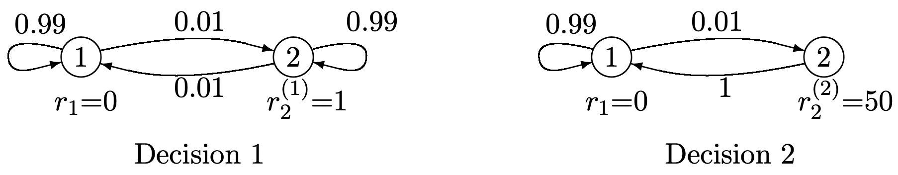 Figure 3.9: A Markov decision problem with two alternatives in state 2.
The set of rules used by the decision maker in selecting an alternative at each time is called a policy. We want to consider the expected aggregate reward over \(n\) steps of the “Markov chain” as a function of the policy used by the decision maker. If for each state \(i\), the policy uses the same decision, say \(k_{i}\), at each occurrence of \(i\), then that policy corresponds to a homogeneous Markov chain with transition probabilities \(P_{i j}^{\left(k_{i}\right)}\). We denote the matrix of these transition probabilities as \(\left[P^{k}\right]\), where \(\boldsymbol{k}=\left(k_{1}, \ldots, k_{\mathrm{M}}\right)\). Such a policy, i.e., mapping each state \(i\) into a fixed decision \(k_{i}\), independent of time and past, is called a stationary policy. The aggregate gain for any such stationary policy was found in the previous section. Since both rewards and transition probabilities depend only on the state and the corresponding decision, and not on time, one feels intuitively that stationary policies make a certain amount of sense over a long period of time. On the other hand, if we look at the example of Figure 3.9, it is clear that decision 2 is the best choice in state 2 at the \(n\)th of \(n\) trials, but it is less obvious what to do at earlier trials.
In what follows, we first derive the optimal policy for maximizing expected aggregate reward over an arbitrary number \(n\) of trials, say at times \(m\) to \(m+n-1\). We shall see that the decision at time \(m+h\), \(0 \leq h<n\), for the optimal policy can in fact depend on \(h\) and \(n\) (but not \(m\)). It turns out to simplify matters considerably if we include a final reward \(\left\{u_{i} ; 1 \leq i \leq \mathrm{M}\right\}\) at time \(m+n\). This final reward \(\boldsymbol{u}\) is considered as a fixed vector, to be chosen as appropriate, rather than as part of the choice of policy.
This optimized strategy, as a function of the number of steps n and the final reward \(\boldsymbol{u}\), is called an optimal dynamic policy for that \(\boldsymbol{u}\). This policy is found from the dynamic programming algorithm, which, as we shall see, is conceptually very simple. We then go on to find the relationship between optimal dynamic policies and optimal stationary policies. We shall find that, under fairly general conditions, each has the same long-term gain per trial.
Dynamic Programming Algorithm
As in our development of Markov chains with rewards, we consider the expected aggregate reward over \(n\) time periods, say \(m\) to \(m+n-1\), with a final reward at time \(m+n\). First consider the optimal decision with \(n=1\). Given \(X_{m}=i\), a decision \(k\) is made with immediate reward \(r_{i}^{(k)}\). With probability \(P_{i j}^{(k)}\) the next state \(X_{m+1}\) is state \(j\) and the final reward is then \(u_{j}\). The expected aggregate reward over times \(m\) and \(m+1\), maximized over the decision \(k\), is then
\[v_{i}^{*}(1, \boldsymbol{u})=\max _{k}\left\{r_{i}^{(k)}+\sum_{j} P_{i j}^{(k)} u_{j}\right\}\label{3.42} \]
Being explicit about the maximizing decision \(k^{\prime}\), \ref{3.42} becomes
\[\begin{gathered}
v_{i}^{*}(1, \boldsymbol{u})=r_{i}^{\left(k^{\prime}\right)}+\sum_{j} P_{i j}^{\left(k^{\prime}\right)} u_{j} \quad \text { for } k^{\prime} \text { such that } \\
r_{i}^{\left(k^{\prime}\right)}+\sum_{j} P_{i j}^{\left(k^{\prime}\right)} u_{j}=\max _{k}\left\{r_{i}^{(k)}+\sum_{j} P_{i j}^{(k)} u_{j}\right\}
\end{gathered}\label{3.43} \]
Note that a decision is made only at time \(m\), but that there are two rewards, one at time \(m\) and the other, the final reward, at time \(m+1\). We use the notation \(v_{i}^{*}(n, \boldsymbol{u})\) to represent the maximum expected aggregate reward from times \(m\) to \(m+n\) starting at \(X_{m}=i\). Decisions (with the reward vector \(\boldsymbol{r}\)) are made at the \(n\) times \(m\) to \(m+n-1\), and this is followed by a final reward vector \(\boldsymbol{u}\) (without any decision) at time \(m+n\). It often simplifies notation to define the vector of maximal expected aggregate rewards
\(\boldsymbol{v}^{*}(n, \boldsymbol{u})=\left(v_{1}^{*}(n, \boldsymbol{u}), v_{2}^{*}(n, \boldsymbol{u}), \ldots, v_{\mathrm{M}}^{*}(1, \boldsymbol{u})\right)^{\top}\).
With this notation, \ref{3.42} and \ref{3.43} become
\[\boldsymbol{v}^{*}(1, \boldsymbol{u})=\max _{\boldsymbol{k}}\left\{\boldsymbol{r}^{k}+\left[P^{\boldsymbol{k}}\right] \boldsymbol{u}\right\} \quad \text { where } \boldsymbol{k}=\left(k_{1}, \ldots, k_{\mathrm{M}}\right)^{\top}, \boldsymbol{r}^{\boldsymbol{k}}=\left(r_{1}^{k_{1}}, \ldots, r_{\mathrm{M}}^{k_{\mathrm{M}}}\right)^{\top}. \label{3.44} \]
\[\boldsymbol{v}^{*}(1, \boldsymbol{u})=\boldsymbol{r}^{k^{\prime}}+\left[P^{k^{\prime}}\right] \boldsymbol{u} \quad \text { where } \boldsymbol{r}^{k^{\prime}}+\left[P^{k^{\prime}}\right] \boldsymbol{u}=\max _{\boldsymbol{k}} \boldsymbol{r}^{k}+\left[P^{k}\right] \boldsymbol{u} .\label{3.45} \]
Now consider \(v_{i}^{*}(2, \boldsymbol{u})\), i.e., the maximal expected aggregate reward starting at \(X_{m}=i\) with decisions made at times \(m\) and \(m+1\) and a final reward at time \(m+2\). The key to dynamic programming is that an optimal decision at time \(m+1\) can be selected based only on the state \(j\) at time \(m+1\); this decision (given \(X_{m+1}=j\)) is optimal independent of the decision at time \(m\). That is, whatever decision is made at time \(m\), the maximal expected reward at times \(m+1\) and \(m+2\), given \(X_{m+1}=j\), is \(\max _{k}\left(r_{j}^{(k)}+\sum_{\ell} P_{j \ell}^{(k)} u_{\ell}\right)\). Note that this maximum is \(v_{j}^{*}(1, \boldsymbol{u})\), as found in (3.42).
Using this optimized decision at time \(m+1\), it is seen that if \(X_{m}=i\) and decision \(k\) is made at time \(m\), then the sum of expected rewards at times \(m+1\) and \(m+2\) is \(\sum_{j} P_{i j}^{(k)} v_{j}^{*}(1, \boldsymbol{u})\). Adding the expected reward at time \(m\) and maximizing over decisions at time \(m\),
\[v_{i}^{*}(2, \boldsymbol{u})=\max _{k}\left(r_{i}^{(k)}+\sum_{j} P_{i j}^{(k)} v_{j}^{*}(1, \boldsymbol{u})\right)\label{3.46} \]
In other words, the maximum aggregate gain over times \(m\) to \(m+2\) (using the final reward \(\boldsymbol{u}\) at \(m+2\)) is the maximum over choices at time \(m\) of the sum of the reward at \(m\) plus the maximum aggregate expected reward for \(m+1\) and \(m+2\). The simple expression of \ref{3.46} results from the fact that the maximization over the choice at time \(m+1\) depends on the state at \(m+1\) but, given that state, is independent of the policy chosen at time \(m\).
This same argument can be used for all larger numbers of trials. To find the maximum expected aggregate reward from time \(m\) to \(m+n\), we first find the maximum expected aggregate reward from \(m+1\) to \(m+n\), conditional on \(X_{m+1}=j\) for each state \(j\). This is the same as the maximum expected aggregate reward from time \(m\) to \(m+n-1\), which is \(v_{j}^{*}(n-1, \boldsymbol{u})\). This gives us the general expression for \(n \geq 2\),
\[v_{i}^{*}(n, \boldsymbol{u})=\max _{k}\left(r_{i}^{(k)}+\sum_{j} P_{i j}^{(k)} v_{j}^{*}(n-1, \boldsymbol{u})\right)\label{3.47} \]
We can also write this in vector form as
\[\boldsymbol{v}^{*}(n, \boldsymbol{u})=\max _{\boldsymbol{k}}\left(\boldsymbol{r}^{\boldsymbol{k}}+\left[P^{\boldsymbol{k}}\right] \boldsymbol{v}^{*}(n-1, \boldsymbol{u})\right)\label{3.48} \]
Here \(\boldsymbol{k}\) is a set (or vector) of decisions, \(\boldsymbol{k}=\left(k_{1}, k_{2}, \ldots, k_{\mathrm{M}}\right)^{\top}\), where \(k_{i}\) is the decision for state \(i\). \(\left[P^{\boldsymbol{k}}\right]\) denotes a matrix whose \((i, j)\) element is \(P_{i j}^{\left(k_{i}\right)}\), and \(\boldsymbol{r}^{\boldsymbol{k}}\) denotes a vector whose \(i\)th element is \(r_{i}^{\left(k_{i}\right)}\). The maximization over \(\boldsymbol{k}\) in \ref{3.48} is really M separate and independent maximizations, one for each state, i.e., \ref{3.48} is simply a vector form of (3.47). Another frequently useful way to rewrite \ref{3.48} is as follows:
\[ \begin{array}{c}\boldsymbol{v}^{*}(n, \boldsymbol{u})=\boldsymbol{r}^{\boldsymbol{k}^{\prime}}+\left[P^{\boldsymbol{k}^{\prime}}\right] \boldsymbol{v}^{*}(n-1, \boldsymbol{u}) \quad \text{ for } \boldsymbol{k}^{\prime}\text{ such that} \\
\boldsymbol{r}^{\boldsymbol{k}^{\prime}}+\left[P^{\boldsymbol{k}^{\prime}}\right] \boldsymbol{v}^{*}(n-1, \boldsymbol{u})=\max _{\boldsymbol{k}}\left(\boldsymbol{r}^{\boldsymbol{k}}+\left[P^{\boldsymbol{k}}\right] \boldsymbol{v}^{*}(n-1, \boldsymbol{u})\right)
\end{array}\label{3.49} \]
If \(\boldsymbol{k}^{\prime}\) satisfies (3.49), then \(\boldsymbol{k}^{\prime}\) is an optimal decision at an arbitrary time \(m\) given, first, that the objective is to maximize the aggregate gain from time \(m\) to \(m+n\), second, that optimal decisions for this objective are to be made at times \(m+1\) to \(m+n-1\), and, third, that \(\boldsymbol{u}\) is the final reward vector at \(m+n\). In the same way, \(\boldsymbol{v}^{*}(n, \boldsymbol{u})\) is the maximum expected reward over this finite sequence of \(n\) decisions from \(m\) to \(m+n-1\) with the final reward \(\boldsymbol{u}\) at \(m+n\).
Note that (3.47), (3.48), and \ref{3.49} are valid with no restrictions (such as recurrent or aperiodic states) on the possible transition probabilities \(\left[P^{\boldsymbol{k}}\right]\). These equations are also valid in principle if the size of the state space is infinite. However, the optimization for each \(n\) can then depend on an infinite number of optimizations at \(n-1\), which is often infeasible.
The dynamic programming algorithm is just the calculation of (3.47), (3.48), or (3.49), performed iteratively for \(n=1,2,3, \ldots\) The development of this algorithm, as a systematic tool for solving this class of problems, is due to Bellman [Bel57]. Note that the algorithm is independent of the starting time \(m\); the parameter \(n\), usually referred to as stage \(n\), is the number of decisions over which the aggregate gain is being optimized. This algorithm yields the optimal dynamic policy for any fixed final reward vector \(\boldsymbol{u}\) and any given number of trials. Along with the calculation of \(\boldsymbol{v}^{*}(n, \boldsymbol{u})\) for each \(n\), the algorithm also yields the optimal decision at each stage (under the assumption that the optimal policy is to be used for each lower numbered stage, i.e., for each later trial of the process).
The surprising simplicity of the algorithm is due to the Markov property. That is, \(v_{i}^{*}(n, \boldsymbol{u})\) is the aggregate present and future reward conditional on the present state. Since it is conditioned on the present state, it is independent of the past (i.e., how the process arrived at state i from previous transitions and choices).
Although dynamic programming is computationally straightforward and convenient13, the asymptotic behavior of \(\boldsymbol{v}^{*}(n, \boldsymbol{u}) as \(n \rightarrow \infty\) is not evident from the algorithm. After working out some simple examples, we look at the general question of asymptotic behavior.
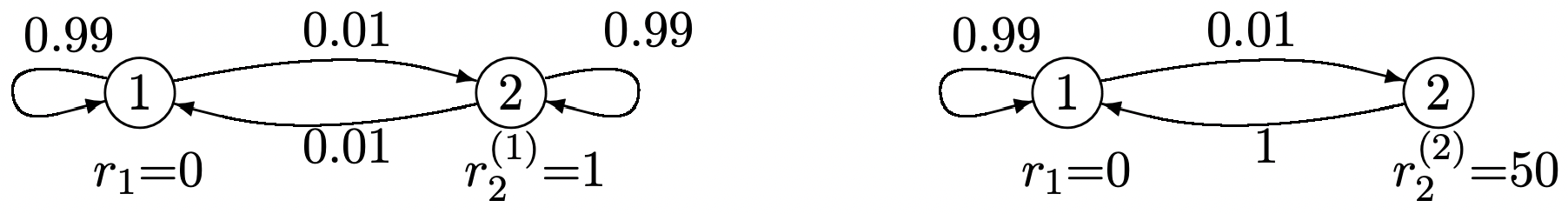
Consider Figure 3.9, repeated below, with the final rewards \(u_{2}=u_{1}=0\).
Solution
Since \(r_{1}=0\) and \(u_{1}=u_{2}=0\), the aggregate gain in state 1 at stage 1 is
\(v_{1}^{*}(1, \boldsymbol{u})=r_{1}+\sum_{j} P_{1 j} u_{j}=0\)
Similarly, since policy 1 has an immediate reward \(r_{2}^{(1)}=1\) in state 2, and policy 2 has an immediate reward \(r_{2}^{(2)}=50\),
\(v_{2}^{*}(1, \boldsymbol{u})=\max \left\{\left[r_{2}^{(1)}+\sum_{j} P_{2 j}^{(1)} u_{j}\right], \quad\left[r_{2}^{(2)}+\sum_{j} P_{2 j}^{(2)} u_{j}\right]\right\}=\max \{1,50\}=50\)
We can now go on to stage 2, using the results above for \(v_{j}^{*}(1, \boldsymbol{u})\). From (3.46),
\(\begin{aligned}
v_{1}^{*}(2, \boldsymbol{u}) &=r_{1}+P_{11} v_{1}^{*}(1, \boldsymbol{u})+P_{12} v_{2}^{*}(1, \boldsymbol{u})=P_{12} v_{2}^{*}(1, \boldsymbol{u})=0.5 \\
v_{2}^{*}(2, \boldsymbol{u}) &=\max \left\{\left[r_{2}^{(1)}+\sum_{j} P_{2 j}^{(1)} v_{j}^{*}(1, \boldsymbol{u})\right], \quad\left[r_{2}^{(2)}+P_{21}^{(2)} v_{1}^{*}(1, \boldsymbol{u})\right]\right\} \\
&=\max \left\{\left[1+P_{22}^{(1)} v_{2}^{*}(1, \boldsymbol{u})\right], 50\right\}=\max \{50.5,50\}=50.5
\end{aligned}\)
Thus for two trials, decision 1 is optimal in state 2 for the first trial (stage 2), and decision 2 is optimal in state 2 for the second trial (stage 1). What is happening is that the choice of decision 2 at stage 1 has made it very profitable to be in state 2 at stage 1. Thus if the chain is in state 2 at stage 2, it is preferable to choose decision 1 (i.e., the small unit gain) at stage 2 with the corresponding high probability of remaining in state 2 at stage 1. Continuing this computation for larger \(n\), one finds that \(v_{1}^{*}(n, \boldsymbol{u})=n / 2\) and \(v_{2}^{*}(n, \boldsymbol{u})=50+n / 2\). The optimum dynamic policy (for \(\boldsymbol{u}=0\)) is decision 2 for stage 1 (i.e., for the last decision to be made) and decision 1 for all stages \(n>1\) (i.e., for all decisions before the last).
This example also illustrates that the maximization of expected gain is not necessarily what is most desirable in all applications. For example, risk-averse people might well prefer decision 2 at the next to final decision (stage 2). This guarantees a reward of 50, rather than taking a small chance of losing that reward.
The problem of finding the shortest paths between nodes in a directed graph arises in many situations, from routing in communication networks to calculating the time to complete complex tasks. The problem is quite similar to the expected first-passage time of example 3.5.1. In that problem, arcs in a directed graph were selected according to a probability distribution, whereas here decisions must be made about which arcs to take. Although this is not a probabilistic problem, the decisions can be posed as choosing a given arc with probability one, thus viewing the problem as a special case of dynamic programming.
Solution
Consider finding the shortest path from each node in a directed graph to some particular node, say node 1 (see Figure 3.10). Each arc (except the special arc (1, 1)) has a positive link length associated with it that might reflect physical distance or an arbitrary type of cost. The special arc (1, 1) has 0 link length. The length of a path is the sum of the lengths of the arcs on that path. In terms of dynamic programming, a policy is a choice of arc out of each node (state). Here we want to minimize cost (i.e., path length) rather than maximizing reward, so we simply replace the maximum in the dynamic programming algorithm with a minimum (or, if one wishes, all costs can be replaced with negative rewards).
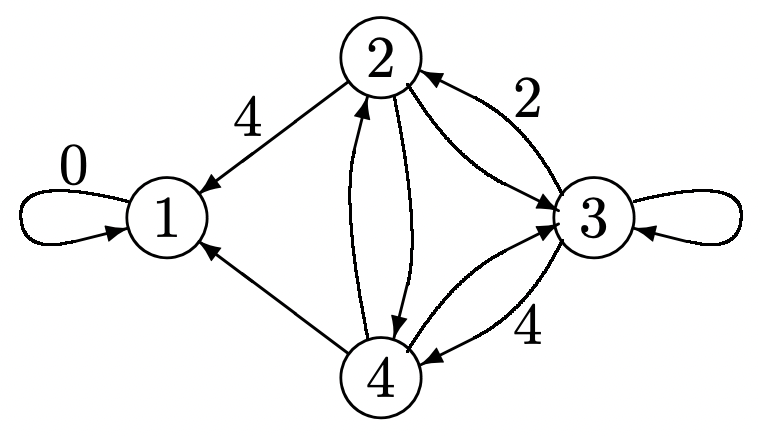 Figure 3.10: A shortest path problem. The arcs are marked with their lengths. Unmarked arcs have unit length.
We start the dynamic programming algorithm with a final cost vector that is 0 for node 1 and infinite for all other nodes. In stage 1, the minimal cost decision for node (state) 2 is arc (2, 1) with a cost equal to 4. The minimal cost decision for node 4 is (4, 1) with unit cost. The cost from node 3 (at stage 1) is infinite whichever decision is made. The stage 1 costs are then
\(v_{1}^{*}(1, \boldsymbol{u})=0, \quad v_{2}^{*}(1, \boldsymbol{u})=4, \quad v_{3}^{*}(1, \boldsymbol{u})=\infty, \quad v_{4}^{*}(1, \boldsymbol{u})=1\)
In stage 2, the cost \(v_{3}^{*}(2, \boldsymbol{u})\), for example, is
\(v_{3}^{*}(2, \boldsymbol{u})=\min \left[2+v_{2}^{*}(1, \boldsymbol{u}), \quad 4+v_{4}^{*}(1, \boldsymbol{u})\right]=5\)
The set of costs at stage 2 are
\(v_{1}^{*}(2, \boldsymbol{u})=0, \quad v_{2}^{*}(2, \boldsymbol{u})=2, \quad v_{3}^{*}(2, \boldsymbol{u})=5, \quad v_{4}^{*}(2, \boldsymbol{u})=1\)
The decision at stage 2 is for node 2 to go to 4, node 3 to 4, and 4 to 1. At stage 3, node 3 switches to node 2, reducing its path length to 4, and nodes 2 and 4 are unchanged. Further iterations yield no change, and the resulting policy is also the optimal stationary policy.
The above results at each stage \(n\) can be interpreted as the shortest paths constrained to at most \(n\) hops. As \(n\) is increased, this constraint is successively relaxed, reaching the true shortest paths in less than M stages.
It can be seen without too much difficulty that these final aggregate costs (path lengths) also result no matter what final cost vector \(\boldsymbol{u}\) (with \(u_{1}=0\)) is used. This is a useful feature for many types of networks where link lengths change very slowly with time and a shortest path algorithm is desired that can track the corresponding changes in the shortest paths.
Optimal stationary policies
In Example 3.6.1, we saw that there was a final transient (at stage 1) in which decision 1 was taken, and in all other stages, decision 2 was taken. Thus, the optimal dynamic policy consisted of a long-term stationary policy, followed by a transient period (for a single stage in this case) over which a different policy was used. It turns out that this final transient can be avoided by choosing an appropriate final reward vector \(\boldsymbol{u}\) for the dynamic programming algorithm. If one has very good intuition, one would guess that the appropriate choice of final reward \(\boldsymbol{u}\) is the relative-gain vector \(\boldsymbol{w}\) associated with the long-term optimal policy.
It seems reasonable to expect this same type of behavior for typical but more complex Markov decision problems. In order to understand this, we start by considering an arbitrary stationary policy \(\boldsymbol{k}^{\prime}=\left(k_{1}^{\prime}, \ldots, k_{\mathrm{M}}^{\prime}\right)\) and denote the transition matrix of the associated Markov chain as \(\left[P^{\boldsymbol{k^{\prime}}}\right]\). We assume that he associated Markov chain is a unichain, or, abbrevating terminology, that \(\boldsymbol{k}^{\prime}\) is a unichain. Let \(\boldsymbol{w}^{\prime}\) be the unique relative-gain vector for \(\boldsymbol{k}^{\prime}\). We then find some necessary conditions for \(\boldsymbol{k}^{\prime}\) to be the optimal dynamic policy at each stage using \(\boldsymbol{w}^{\prime}\) as the final reward vector.
First, from \ref{3.45} \(\boldsymbol{k}^{\prime}\) is an optimal dynamic decision (with the final reward vector \(\boldsymbol{w}^{\prime}\) for \(\left[P^{\boldsymbol{k^{\prime}}}\right]\)) at stage 1 if
\[\boldsymbol{r^{k^{\prime}}}+\left[\boldsymbol{P^{k^{\prime}}}\right] \boldsymbol{w}^{\prime}=\max _{\boldsymbol{k}}\left\{\boldsymbol{r^{k}}+\left[\boldsymbol{P^{k}}\right] \boldsymbol{w}^{\prime}\right\}\label{3.50} \]
Note that this is more than a simple statement that \(\boldsymbol{k}^{\prime}\) can be found by maximizing \(\boldsymbol{r^k}+\left[P^{ \boldsymbol{k}}\right] \boldsymbol{w}^{\prime}\) over \(\boldsymbol{k}\). It also involves the fact that \(\boldsymbol{w}^{\prime}\) is the relative-gain vector for \(\boldsymbol{k}^{\prime}\), so there is no immediately obvious way to find a \(\boldsymbol{k}^{\prime}\) that satisfies (3.50), and no a priori assurance that this equation even has a solution. The following theorem, however, says that this is the only condition required to ensure that \(\boldsymbol{k}^{\prime}\) is the optimal dynamic policy at every stage (again using \(\boldsymbol{w}^{\prime}\) as the final reward vector).
Assume that \ref{3.50} is satisfied for some policy \(\boldsymbol{k}^{\prime}\) where the Markov chain for \(\boldsymbol{k}^{\prime}\) is a unichain and \(\boldsymbol{w}^{\prime}\) is the relative-gain vector of \(\boldsymbol{k}^{\prime}\). Then the optimal dynamic policy, using \(\boldsymbol{w}^{\prime}\) as the final reward vector, is the stationary policy \(\boldsymbol{k}^{\prime}\). Furthermore the optimal gain at each stage \(n\) is given by
\[\boldsymbol{v}^{*}\left(n, \boldsymbol{w}^{\prime}\right)=\boldsymbol{w}^{\prime}+n g^{\prime} \boldsymbol{e}\label{3.51} \]
where \(g^{\prime}=\boldsymbol{\pi}^{\prime} \boldsymbol{r}^{\boldsymbol{k}^{\prime}}\) and \(\boldsymbol{\pi^{\prime}}\) is the steady-state vector for \(\boldsymbol{k}^{\prime}\).
- Proof
-
We have seen from \ref{3.45} that \(\boldsymbol{k}^{\prime}\) is an optimal dynamic decision at stage 1. Also, since \(\boldsymbol{w}^{\prime}\) is the relative-gain vector for \(\boldsymbol{k}^{\prime}\), Theorem 3.5.2 asserts that if decision \(\boldsymbol{k}^{\prime}\) is used at each stage, then the aggregate gain satisfies \(\boldsymbol{v}\left(n, \boldsymbol{w}^{\prime}\right)=n g^{\prime} \boldsymbol{e}+\boldsymbol{w}^{\prime}\). Since \(\boldsymbol{k}^{\prime}\) is optimal at stage 1, it follows that \ref{3.51} is satisfied for \(n=1\).
We now use induction on \(n\), with \(n=1\) as a basis, to verify \ref{3.51} and the optimality of this same \(\boldsymbol{k}^{\prime}\) at each stage \(n\). Thus, assume that \ref{3.51} is satisfied for \(n\). Then, from (3.48),
\(\begin{aligned}
\boldsymbol{v}^{*}\left(n+1, \boldsymbol{w}^{\prime}\right) &=\max _{\boldsymbol{k}}\left\{\boldsymbol{r}^{\boldsymbol{k}}+\left[\boldsymbol{P^{k}}\right] \boldsymbol{v}^{*}\left(n, \boldsymbol{w}^{\prime}\right)\right\} &(3.52)\\
&=\max _{\boldsymbol{k}}\left\{\boldsymbol{r}^{\boldsymbol{k}}+\left[\boldsymbol{P^{\boldsymbol{k}}}\right]\left\{\boldsymbol{w}^{\prime}+n g^{\prime} \boldsymbol{e}\right\}\right\}&(3.53) \\
&=n g^{\prime} \boldsymbol{e}+\max _{\boldsymbol{k}}\left\{\boldsymbol{r}^{\boldsymbol{k}}+\left[\boldsymbol{P^{k}}\right] \boldsymbol{w}^{\prime}\right\} &(3.54)\\
&\left.=n g^{\prime} \boldsymbol{e}+\boldsymbol{r}^{\boldsymbol{k}^{\prime}}+\left[\boldsymbol{P^{k^\prime}}\right] \boldsymbol{w}^{\prime}\right\} &(3.55)\\
&=(n+1) g^{\prime} \boldsymbol{e}+\boldsymbol{w}^{\prime} .&(3.56)
\end{aligned}\)
Eqn \ref{3.53} follows from the inductive hypothesis of (3.51), \ref{3.54} follows because \(\left[P^{\boldsymbol{k}}\right] \boldsymbol{e}=\boldsymbol{e}\) for all \(\boldsymbol{k}\), \ref{3.55} follows from (3.50), and \ref{3.56} follows from the definition of \(\boldsymbol{w}^{\prime}\) as the relative-gain vector for \(\boldsymbol{k}^{\prime}\). This verifies \ref{3.51} for \(n+1\). Also, since \(\boldsymbol{k}^{\prime}\) maximizes (3.54), it also maximizes (3.52), showing that \(\boldsymbol{k}^{\prime}\) is the optimal dynamic decision at stage \(n+1\). This completes the inductive step.
Since our major interest in stationary policies is to help understand the relationship between the optimal dynamic policy and stationary policies, we define an optimal stationary policy as follows:
A unichain stationary policy \(\boldsymbol{k}^{\prime}\) is optimal if the optimal dynamic policy with \(\boldsymbol{w}^{\prime}\) as the final reward uses \(\boldsymbol{k}^{\prime}\) at each stage.
This definition side-steps several important issues. First, we might be interested in dynamic programming for some other final reward vector. Is it possible that dynamic programming performs much better in some sense with a different final reward vector. Is it possible that there is another stationary policy, especially one with a larger gain per stage? We answer these questions later and find that stationary policies that are optimal according to the definition do have maximal gain per stage compared with dynamic policies with arbitrary final reward vectors.
From Theorem 3.6.1, we see that if there is a policy \(\boldsymbol{k}^{\prime}\) which is a unichain with relative-gain vector \(\boldsymbol{w}^{\prime}\), and if that \(\boldsymbol{k}^{\prime}\) is a solution to (3.50), then \(\boldsymbol{k}^{\prime}\) is an optimal stationary policy.
It is easy to imagine Markov decision models for which each policy corresponds to a Markov chain with multiple recurrent classes. There are many special cases of such situations, and their detailed study is inappropriate in an introductory treatment. The essential problem with such models is that it is possible to get into various sets of states from which there is no exit, no matter what decisions are used. These sets might have different gains, so that there is no meaningful overall gain per stage. We avoid these situations by a modeling assumption called inherent reachability, which assumes, for each pair \((i, j)\) of states, that there is some decision vector \(\boldsymbol{k}\) containing a path from \(i\) to \(j\).
The concept of inherent reachability is a little tricky, since it does not say the same \(\boldsymbol{k}\) can be used for all pairs of states (i.e., that there is some \(\boldsymbol{k}\) for which the Markov chain is recurrent). As shown in Exercise 3.31, however, inherent reachability does imply that for any state \(j\), there is a \(\boldsymbol{k}\) for which \(j\) is accessible from all other states. As we have seen a number of times, this implies that the Markov chain for \(\boldsymbol{k}\) is a unichain in which \(j\) is a recurrent state.
Any desired model can be modified to satisfy inherent reachability by creating some new decisions with very large negative rewards; these allow for such paths but very much discourage them. This will allow us to construct optimal unichain policies, but also to use the appearance of these large negative rewards to signal that there was something questionable in the original model.
Policy improvement and the seach for optimal stationary policies
The general idea of policy improvement is to start with an arbitrary unichain stationary policy \(\boldsymbol{k}^{\prime}\) with a relative gain vector \(\boldsymbol{w}^{\prime}\) (as given by (3.37)). We assume inherent reachability throughout this section, so such unichains must exist. We then check whether (3.50), is satisfied, and if so, we know from Theorem 3.6.1 that \(\boldsymbol{k}^{\prime}\) is an optimal stationary policy. If not, we find another stationary policy \(\boldsymbol{k}\) that is ‘better’ than \(\boldsymbol{k}^{\prime}\) in a sense to be described later. Unfortunately, the ‘better’ policy that we find might not be a unichain, so it will also be necessary to convert this new policy into an equally ‘good’ unichain policy. This is where the assumption of of inherent reachability is needed. The algorithm then iteratively finds better and better unichain stationary policies, until eventually one of them satisfies \ref{3.50} and is thus optimal.
We now state the policy-improvement algorithm for inherently reachable Markov decision problems. This algorithm is a generalization of Howard’s policy-improvement algorithm, [How60].
Policy-improvement Algorithm
- Choose an arbitrary unichain policy \(\boldsymbol{k}^{\prime}\)
- For policy \(\boldsymbol{k}^{\prime}\), calculate \(\boldsymbol{w}^{\prime}\) and \(g^{\prime}\) from \(\boldsymbol{w}^{\prime}+g^{\prime} \boldsymbol{e}=\boldsymbol{r}^{\boldsymbol{k}^{\prime}}+\left[P^{\boldsymbol{k}^{\prime}}\right] \boldsymbol{w}^{\prime}\) and \(\boldsymbol{\pi}^{\prime} \boldsymbol{w}^{\prime}=0\).
- If \(\boldsymbol{r}^{\boldsymbol{k}^{\prime}}+\left[P^{\boldsymbol{k}^{\prime}}\right] \boldsymbol{w}^{\prime}=\max _{\boldsymbol{k}}\left\{\boldsymbol{r}^{\boldsymbol{k}}+\left[P^{\boldsymbol{k}}\right] \boldsymbol{w}^{\prime}\right\}\), then stop; \(\boldsymbol{k}^{\prime}\) is optimal.
- Otherwise, choose \(\ell\) and \(k_{\ell}\) so that \(r_{\ell}^{\left(k_{\ell}^{\prime}\right)}+\sum_{j} P_{\ell j}^{\left(k_{\ell}^{\prime}\right)} w_{j}^{\prime}<r_{\ell}^{\left(k_{\ell}\right)}+\sum_{j} P_{\ell j}^{\left(k_{\ell}\right)} w_{j}^{\prime}\). For \(i \neq \ell\), let \(k_{i}=k_{i}^{\prime}\).
- If \(\boldsymbol{k}=\left(k_{1}, \ldots k_{\mathrm{M}}\right)\) is not a unichain, then let \(\mathcal{R}\) be the recurrent class in \(\boldsymbol{k}\) that contains state \(\ell\), and let \(\tilde{\boldsymbol{k}}\) be a unichain policy for which \(\tilde{k}_{i}=k_{i}\) for each \(i \in \mathcal{R}\). Alternatively, if \(\boldsymbol{k} \) is already a unichain, let \(\tilde{\boldsymbol{k}}=\boldsymbol{k}\).
- Update \(\boldsymbol{k}^{\prime}\) to the value of \(\tilde{\boldsymbol{k}}\) and return to step 2.
If the stopping test in step 3 fails, there must be an \(\ell\) and \(k_{\ell}\) for which \(r_{\ell}^{\left(k_{\ell}^{\prime}\right)}+\sum_{j} P_{\ell j}^{\left(k_{\ell}^{\prime}\right)} w_{j}^{\prime}< r_{\ell}^{\left(k_{\ell}\right)}+\sum_{j} P_{\ell j}^{\left(k_{\ell}\right)} w_{j}^{\prime}\). Thus step 4 can always be executed if the algorithm does not stop in step 3, and since the decision is changed only for the single state \(\ell\), the resulting policy \(\boldsymbol{k}\) satisfies
\[\boldsymbol{r}^{\boldsymbol{k}^{\prime}}+\left[p^{\boldsymbol{k}^{\prime}}\right] \boldsymbol{\boldsymbol { w }}^{\prime} \leq \boldsymbol{r}^{\boldsymbol{k}}+\left[P^{\boldsymbol{k}}\right] \boldsymbol{w}^{\prime} \quad \text { with strict inequality for component } \ell\label{3.57} \]
The next three lemmas consider the different cases for the state \(\ell\) whose decision is changed in step 4 of the algorithm. Taken together, they show that each iteration of the algorithm either increases the gain per stage or keeps the gain per stage constant while increasing the relative gain vector. After proving these lemmas, we return to show that the algorithm must converge and explain the sense in which the resulting stationary algorithm is optimal.
For each of the lemmas, let \(\boldsymbol{k}^{\prime}\) be the decision vector in step 1 of a given iteration of the policy improvement algorithm and assume that the Markov chain for \(\boldsymbol{k}^{\prime}\) is a unichain. Let \(g^{\prime}, \boldsymbol{w}^{\prime}\), and \(\mathcal{R}^{\prime}\) respectively be the gain per stage, the relative gain vector, and the recurrent set of states for \(\boldsymbol{k}^{\prime}\). Assume that the stopping condition in step 3 is not satisfied and that \(\ell\) denotes the state whose decision is changed. Let \(k_{\ell}\) be the new decision in step 4 and let \(\boldsymbol{k}\) be the new decision vector.
Assume that \(\ell \in \mathcal{R}^{\prime}\). Then the Markov chain for \(\boldsymbol{k}\) is a unichain and \(\ell\) is recurrent in \(\boldsymbol{k}\). The gain per stage g for \(\boldsymbol{k}\) satisfies \(g>g^{\prime}\).
- Proof
-
The Markov chain for \(\boldsymbol{k}\) is the same as that for \(\boldsymbol{k}^{\prime}\) except for the transitions out of state \(\ell\). Thus every path into \(\ell\) in \(\boldsymbol{k}^{\prime}\) is still a path into \(\ell\) in \(\boldsymbol{k}\). Since \(\ell\) is recurrent in the unichain \(\boldsymbol{k}^{\prime}\), it is accessible from all states in \(\boldsymbol{k}^{\prime}\) and thus in \(\boldsymbol{k}\). It follows (see Exercise 3.3) that \(\ell\) is recurrent in \(\boldsymbol{k}\) and \(\boldsymbol{k}\) is a unichain. Since \(\boldsymbol{r}^{\boldsymbol{k}^{\prime}}+\left[P^{\boldsymbol{k}^{\prime}}\right] \boldsymbol{w}^{\prime}=\boldsymbol{w}^{\prime}+g^{\prime} \boldsymbol{e}\) (see (3.37)), we can rewrite \ref{3.57} as
\[\boldsymbol{w}^{\prime}+g^{\prime} \boldsymbol{e} \leq \boldsymbol{r}^{k}+\left[P^{k}\right] \boldsymbol{w}^{\prime} \quad \text { with strict inequality for component } \ell\label{3.58} \]
Premultiplying both sides of \ref{3.58} by the steady-state vector \(\pi\) of the Markov chain \(\boldsymbol{k}\) and using the fact that \(\ell\) is recurent and thus \(\pi_{\ell}>0\),
\(\boldsymbol{\pi} \boldsymbol{w}^{\prime}+g^{\prime}<\boldsymbol{\pi} \boldsymbol{r^{k}}+\boldsymbol{\pi}\left[\boldsymbol{P^{k}}\right] \boldsymbol{w}^{\prime}\)
Since \(\boldsymbol{\pi}\left[\boldsymbol{P^{k}}\right]=\boldsymbol{\pi}\), this simplifies to
\[g^{\prime}<\boldsymbol{\pi} \boldsymbol{r}^{k}\label{3.59} \]
The gain per stage \(g\) for \(\boldsymbol{k}\) is \(\boldsymbol{\pi r^{k}}\), so we have \(g^{\prime}<g\).
Assume that \(\ell \notin \mathcal{R}^{\prime}\) (i.e., \(\ell\) is transient in \(\boldsymbol{k}^{\prime}\)) and that the states of \(\mathcal{R}^{\prime}\) are not accessible from \(\ell\) in \(\boldsymbol{k}\). Then \(\boldsymbol{k}\) is not a unichain and \(\ell\) is recurrent in \(\boldsymbol{k}\). A decision vector \(\tilde{\boldsymbol{k}}\) exists that is a unichain for which \(\tilde{k}_{i}=k_{i}\) for \(i \in \mathcal{R}\), and its gain per stage \(\tilde{g}\) satisfies \(\tilde{g}>g\).
- Proof
-
Since \(\ell \notin \mathcal{R}^{\prime}\), the transition probabilities from the states of \(\mathcal{R}^{\prime}\) are unchanged in going from \(\boldsymbol{k}^{\prime}\) to \(\boldsymbol{k}\). Thus the set of states accessible from \(\mathcal{R}^{\prime}\) remains unchanged, and \(\mathcal{R}^{\prime}\) is a recurrent set of \(\boldsymbol{k}\). Since \(\mathcal{R}^{\prime}\) is not accessible from \(\ell\), there must be another recurrent set, \(\mathcal{R}\), in \(\boldsymbol{k}\), and thus \(\boldsymbol{k}\) is not a unichain. The states accessible from \(\mathcal{R}\) no longer include \(\mathcal{R}^{\prime}\), and since \(\ell\) is the only state whose transition probabilities have changed, all states in \(\mathcal{R}\) have paths to \(\ell\) in \(\boldsymbol{k}\). It follows that \(\ell \in \mathcal{R}\).
Now let \(\boldsymbol{\pi}\) be the steady-state vector for \(\mathcal{R}\) in the Markov chain for \(\boldsymbol{k}\). Since \(\pi_{\ell}>0\), \ref{3.58} and \ref{3.59} are still valid for this situation. Let \(\tilde{\boldsymbol{k}}\) be a decision vector for which \(\tilde{k}_{i}=k_{i}\) for each \(i \in \mathcal{R}\). Using inherent reachability, we can also choose \(\tilde{k}_{i}\) for each \(i \notin \mathcal{R}\) so that \(\ell\) is reachable from \(i\) (see Exercise 3.31). Thus \(\tilde{\boldsymbol{k}}\) is a unichain with the recurrent class \(\mathcal{R}\). Since \(\tilde{\boldsymbol{k}}\) has the same transition probabilities and rewards in \(\mathcal{R}\) as \(\boldsymbol{k}\), we see that \(\tilde{g}=\pi \boldsymbol{r}^{\boldsymbol{k}}\) and thus \(\tilde{g}>g^{\prime}\).
The final lemma now includes all cases not in Lemmas 3.6.1 and 3.6.2
Assume that \(\ell \notin \mathcal{R}^{\prime}\) and that \(\mathcal{R}^{\prime}\) is accessible from \(\ell\) in \(\boldsymbol{k}\). Then \(\boldsymbol{k}\) is a unichain with the same recurrent set \(\mathcal{R}^{\prime}\) as \(\boldsymbol{k}^{\prime}\). The gain per stage \(g\) is equal to \(g^{\prime}\) and the relative-gain vector \(\boldsymbol{w}\) of \(\boldsymbol{k}\) satisfies
\[\boldsymbol{w}^{\prime} \leq \boldsymbol{w} \quad \text { with } w_{\ell}^{\prime}<w_{\ell} \text { and } w_{i}^{\prime}=w_{i} \text { for } i \in \mathcal{R}^{\prime}\label{3.60} \]
- Proof
-
Since \(\boldsymbol{k}^{\prime}\) is a unichain, \(\boldsymbol{k}^{\prime}\) contains a path from each state to \(\mathcal{R}^{\prime}\). If such a path does not go through state \(\ell\), then \(\boldsymbol{k}\) also contains that path. If such a path does go through \(\ell\), then that path can be replaced in \(\boldsymbol{k}\) by the same path to \(\ell\) followed by a path in \(\boldsymbol{k}\) from \(\ell\) to \(\mathcal{R}^{\prime}\). Thus \(\mathcal{R}^{\prime}\) is accessible from all states in \(\boldsymbol{k}\). Since the states accessible from \(\mathcal{R}^{\prime}\) are unchanged from \(\boldsymbol{k}^{\prime}\) to \(\boldsymbol{k}\), \(\boldsymbol{k}\) is still a unichain with the recurrent set \(\mathcal{R}^{\prime}\) and state \(\ell\) is still transient.
If we write out the defining equation \ref{3.37} for \(\boldsymbol{w}^{\prime}\) component by component, we get
\[w_{i}^{\prime}+g^{\prime}=r_{i}^{k_{i}^{\prime}}+\sum_{j} P_{i j}^{k_{i}^{\prime}} w_{j}^{\prime}\label{3.61} \]
Consider i the set of these equations for which \(i \in \mathcal{R}^{\prime}\). Since \(P_{i j}^{k_{i}^{\prime}}=0\) for all transient \(j\) in \(\boldsymbol{k}^{\prime}\), these are the same relative-gain equations as for the Markov chain restricted to \(\mathcal{R}^{\prime}\). Therefore \(\boldsymbol{w}^{\prime}\) is uniquely defined for \(i \in \mathcal{R}_{i}^{\prime}\) by this restricted set of equations. These equations are not changed in going from \(\boldsymbol{k}^{\prime}\) to \(\boldsymbol{k}\), so it follows that \(w_{i}=w_{i}^{\prime}\) for \(i \in \mathcal{R}^{\prime}\). We have also seen that the steady-state vector \(\boldsymbol{\pi}^{\prime}\) is determined solely by the transition probabilities in the recurrent class, so \(\boldsymbol{\pi}^{\prime}\) is unchanged from \(\boldsymbol{k}^{\prime}\) to \(\boldsymbol{k}\), and \(g=g^{\prime}\).
Finally, consider the difference between the relative-gain equations for \(\boldsymbol{k}^{\prime}\) in 3.61 and those for \(\boldsymbol{k}\). Since \(g^{\prime}=g\),
\[w_{i}-w_{i}^{\prime}=r_{i}^{k_{i}}-r_{i}^{k_{i}^{\prime}}+\sum_{j}\left(P_{i j}^{k_{i}} w_{j}-P_{i j}^{k_{i}^{\prime}} w_{j}^{\prime}\right)\label{3.62} \]
For all \(i \neq \ell\), this simplifies to
\[w_{i}-w_{i}^{\prime}=\sum_{j} P_{i j}^{k_{i}}\left(w_{j}-w_{j}^{\prime}\right)\label{3.63} \]
For \(i=\ell\), \ref{3.62} can be rewritten as
\[w_{\ell}-w_{\ell}^{\prime}=\sum_{j} P_{\ell j}^{k_{\ell}}\left(w_{j}-w_{j}^{\prime}\right)+\left[r_{\ell}^{k_{\ell}}-r_{\ell}^{k_{\ell}^{\prime}}+\sum_{j}\left(P_{\ell j}^{k_{\ell}} w_{j}^{\prime}-P_{\ell j}^{k_{\ell}^{\prime}} w_{j}^{\prime}\right)\right]\label{3.64} \]
The quantity in brackets must be positive because of step 4 of the algorithm, and we denote it as \(\hat{r}_{\ell}-\hat{r}_{\ell}^{\prime}\). If we also define \(\hat{r}_{i}=\hat{r}_{i}^{\prime}\) for \(i \neq \ell\), then we can apply the last part of Corollary 3.5.1 (using \(\hat{\boldsymbol{r}}\) and \(\hat{\boldsymbol{r}}^{\prime}\) as reward vectors) to conclude that \(\boldsymbol{w} \geq \boldsymbol{w}^{\prime}\) with \(w_{\ell}>w_{\ell}^{\prime}\).
We now see that each iteration of the algorithm either increases the gain per stage or holds the gain per stage the same and increases the relative-gain vector \(\boldsymbol{w}\). Thus the sequence of policies found by the algorithm can never repeat. Since there are a finite number of stationary policies, the algorithm must eventually terminate at step 3. This means that the optimal dynamic policy using the final reward vector \(\boldsymbol{w}^{\prime}\) for the terminating decision vector \(\boldsymbol{k}^{\prime}\) must in fact be the stationary policy \(\boldsymbol{k}^{\prime}\).
The question now arises whether the optimal dynamic policy using some other final reward vector can be substantially better than that using \(\boldsymbol{w}^{\prime}\). The answer is quite simple and is developed in Exercise 3.30. It is shown there that if \(\boldsymbol{u}\) and \(\boldsymbol{u}^{\prime}\) are arbitrary final reward vectors used on the dynamic programming algorithm, then \(v^{*}(n, \boldsymbol{u})\) and \(v^{*}\left(n, \boldsymbol{u}^{\prime}\right)\) are related by
\(v^{*}(n, \boldsymbol{u}) \leq v^{*}\left(n, \boldsymbol{u}^{\prime}\right)+\alpha \boldsymbol{e},\)
where \(\alpha=\max _{i}\left(u_{i}-u_{i}^{\prime}\right)\). Using \(\boldsymbol{w}^{\prime}\) for \(\boldsymbol{u}^{\prime}\), it is seen that the gain per stage of dynamic i programming, with any final reward vector, is at most the gain \(g^{\prime}\) of the stationary policy at the termination of the policy-improvement algorithm.
The above results are summarized in the following theorem.
For any inherently reachable finite-state Markov decision problem, the policy-improvement algorithm terminates with a stationary policy \(\boldsymbol{k}^{\prime}\) that is the same as the solution to the dynamic programming algorithm using \(\boldsymbol{w}^{\prime}\) as the final reward vector. The gain per stage \(g^{\prime}\) of this stationary policy maximizes the gain per stage over all stationary policies and over all final-reward vectors for the dynamic programming algorithm.
One remaining issue is the question whether the relative-gain vector found by the policyimprovement algorithm is in any sense optimal. The example in Figure 3.11 illustrates two different solutions terminating the policy-improvement algorithm. They each have the same gain (as guaranteed by Theorem 3.6.2) but their relative-gain vectors are not ordered.
In many applications such as variations on the shortest path problem, the interesting issue is what happens before the recurrent class is entered, and there is often only one recurrent class and one set of decisions within that class of interest. The following corollary shows that in this case, the relative-gain vector for the stationary policy that terminates the algorithm is maximal not only among the policies visited by the algorithm but among all policies with the same recurrent class and the same decisions within that class. The proof is almost the same as that of Lemma 3.6.3 and is carried out in Exercise 3.33.
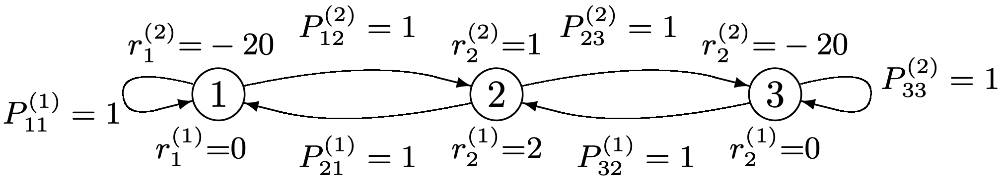 Figure 3.11: A Markov decision problem in which there are two unichain decision vectors (one left-going, and the other right-going). For each, \ref{3.50} is satisfied and the gain per stage is 0. The dynamic programming algorithm (with no final reward) is stationary but has two recurrent classes, one of which is {3}, using decision 2 and the other of which is {1, 2}, using decision 1 in each state.
Assume the policy improvement algorithm terminates with the recurrent class \(\mathcal{R}^{\prime}\), the decision vector \(\boldsymbol{k}^{\prime}\), and the relative-gain vector \(\boldsymbol{w}^{\prime}\). Then for any stationary policy that has the recurrent class \(\mathcal{R}^{\prime}\) and a decision vector \(\boldsymbol{k}\) satisfying \(k_{i}=k_{i}^{\prime}\) for all \(i \in \mathcal{R}^{\prime}\), the relative gain vector \(\boldsymbol{w}\) satisfies \(\boldsymbol{w} \leq \boldsymbol{w}^{\prime}\).
Reference
13Unfortunately, many dynamic programming problems of interest have enormous numbers of states and possible choices of decision (the so called curse of dimensionality), and thus, even though the equations are simple, the computational requirements might be beyond the range of practical feasibility.