4.5: Random Stopping Trials

Visualize performing an experiment repeatedly, observing independent successive sample outputs of a given random variable (i.e., observing a sample outcome of \(X_{1}, X_{2}, \ldots\) where the \(X_{i}\) are IID). The experiment is stopped when enough data has been accumulated for the purposes at hand.

This type of situation occurs frequently in applications. For example, we might be required to make a choice from several hypotheses, and might repeat an experiment until the hypotheses are sufficiently discriminated. If the number of trials is allowed to depend on the outcome, the mean number of trials required to achieve a given error probability is typically a small fraction of the number of trials required when the number is chosen in advance. Another example occurs in tree searches where a path is explored until further extensions of the path appear to be unprofitable.

The first careful study of experimental situations where the number of trials depends on the data was made by the statistician Abraham Wald and led to the field of sequential analysis (see [21]). We study these situations now since one of the major results, Wald’s equality, will be useful in studying \(\mathrm{E}[N(t)]\) in the next section. Stopping trials are frequently useful in the study of random processes, and in particular will be used in Section 4.7 for the analysis of queues, and again in Chapter 7 as central topics in the study of Random walks and martingales.

An important part of experiments that stop after a random number of trials is the rule for stopping. Such a rule must specify, for each sample path, the trial at which the experiment stops, i.e., the final trial after which no more trials are performed. Thus the rule for stopping should specify a positive, integer valued, random variable \(J\), called the stopping time, or stopping trial, mapping sample paths to this final trial at which the experiment stops.

We view the sample space as including the set of sample value sequences for the never-ending sequence of random variables \(X_{1}, X_{2}, \ldots\). That is, even if the experiment is stopped at the end of the second trial, we still visualize the 3rd, 4th, . . . random variables as having sample values as part of the sample function. In other words, we visualize that the experiment continues forever, but that the observer stops watching at the end of the stopping point. From the standpoint of applications, the experiment might or might not continue after the observer stops watching. From a mathematical standpoint, however, it is far preferable to view the experiment as continuing. This avoids confusion and ambiguity about the meaning of IID rv’s when the very existence of later variables depends on earlier sample values.

The intuitive notion of stopping a sequential experiment should involve stopping based on the data (i.e., the sample values) gathered up to and including the stopping point. For example, if \(X_{1}, X_{2}, \ldots\), represent the succesive changes in our fortune when gambling, we might want to stop when our cumulative gain exceeds some fixed value. The stopping trial \(n\) then depends on the sample values of \(X_{1}, X_{2}, \ldots, X_{n}\). At the same time, we want to exclude from stopping trials those rules that allow the experimenter to peek at subsequent values before making the decision to stop or not.⁸ This leads to the following definition.

Definition 4.5.1

A stopping trial (or stopping time⁹) J for a sequence of rv’s \(X_{1}, X_{2}, \ldots\), is a positive integer-valued rv such that for each \(n \geq 1\), the indicator rv \(\mathbb{I}_{\{J=n\}}\) is a function of \(\left\{X_{1}, X_{2}, \ldots, X_{n}\right\}\).

The last clause of the definition means that any given sample value \(x_{1}, \ldots, x_{n}\) for \(X_{1}, \ldots, X_{n}\) uniquely determines whether the corresponding sample value of \(J\) is defined to be a positive integer-valued rv, the events \(\{J=n\}\) and \(\{J=m\}\) for \(m<n\) are disjoint events, so stopping at trial \(m\) makes it impossible to also stop at \(n\) for a given sample path. Also the union of the events \(\{J=n\}\) over \(n \geq 1\) has probability 1. Aside from this final restriction, the definition does not depend on the probability measure and depends solely on the set of events \(\{J=n\}\) for each \(n\). In many situations, it is useful to relax the definition further to allow \(J\) to be a possibly-defective rv. In this case the question of whether stopping occurs with probability 1 can be postponed until after specifying the disjoint events \(\{J=n\}\) over \(n \geq 1\).

Example 4.5.1

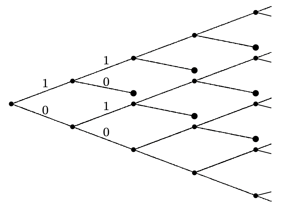
Consider a Bernoulli process \(\left\{X_{n} ; n \geq 1\right\}\). A very simple stopping trial for this process is to stop at the first occurrence of the string (1, 0). Figure 4.11 illustrates this stopping trial by viewing it as a truncation of the tree of possible binary sequences.

The event \(\{J=2\}\), i.e., the event that stopping occurs at trial 2, is the event \(\left\{X_{1}=1, X_{2}=0\right\}\). Similarly, the event \(\{J=3\}\) is \(\left\{X_{1}=1, X_{2}=1, X_{3}=0\right\} \bigcup\left\{X_{1}=0, X_{2}=1, X_{3}=0\right\}\). The disjointness of \(\{J=n\}\) and \(\{J=m\}\) for \(n \neq m\) is represented in the figure by terminating the tree at each stopping node. It can be seen that the tree never dies out completely, and in fact, for each trial \(n\), the number of stopping nodes is \(n-1\). However, the probability that stopping has not occurred by trial \(n\) goes to zero exponentially with \(n\), which ensures that \(J\) is a random variable.

Figure 4.11: A tree representing the set of binary sequences, with a stopping rule viewed as a pruning of the tree. The particular stopping rule here is to stop on the first occurrence of the string (1, 0). The leaves of the tree (i.e., the nodes at which stopping occurs) are marked with large dots and the intermediate nodes (the other nodes) with small dots. Note that each leaf in the tree has a one-to-one correspondence with an initial segment of the tree, so the stopping nodes can be unambiguously viewed either as leaves of the tree or initial segments of the sample sequences.

Representing a stopping rule by a pruned tree can be used for any discrete random sequence, although the tree becomes quite unwieldy in all but trivial cases. Visualizing a stopping rule in terms of a pruned tree is useful conceptually, but stopping rules are usually stated in other terms. For example, we shortly consider a stopping trial for the interarrival intervals of a renewal process as the first \(n\) for which the arrival epoch \(S_{n}\) satisfies \(S_{n}>t\) for some given \(t>0\).

Wald’s equality

An important question that arises with stopping trials is to evaluate the sum \(S_{J}\) of the random variables up to the stopping trial, i.e., \(S_{J}=\sum_{n=1}^{J} X_{n}\). Many gambling strategies and investing strategies involve some sort of rule for when to stop, and it is important to understand the rv \(S_{J}\) (which can model the overall gain or loss up to that trial). Wald’s equality is very useful in helping to find \(\mathrm{E}\left[S_{J}\right]\).

Theorem 4.5.1: Wald's Equality

Let \(\left\{X_{n} ; n \geq 1\right\}\) be a sequence of IID rv’s, each of mean \(\bar{X}\). If \(J\) is a stopping trial for \(\left\{X_{n} ; n \geq 1\right\}\) and if \(\mathrm{E}[J]<\infty\), then the sum \(S_{J}=X_{1}+X_{2}+\cdots+X_{J}\) at the stopping trial \(J\) satisfies

\[\mathrm{E}\left[S_{J}\right]=\bar{X} \mathrm{E}[J]\label{4.30} \]

Proof

Note that \(X_{n}\) is included in \(S_{J}=\sum_{n=1}^{J} X_{n}\) whenever \(n \leq J\), i.e., whenever the n=1 indicator function \(\mathbb{I}_{\{J \geq n\}}=1\). Thus

\[S_{J}=\sum_{n=1}^{\infty} X_{n} \mathbb{I}_{\{J \geq n\}}\label{4.31} \]

This includes \(X_{n}\) as part of the sum if stopping has not occurred before trial \(n\). The event \(\{J \geq n\}\) is the complement of \(\{J<n\}=\{J=1\} \bigcup \cdots \bigcup\{J=n-1\}\). All of these latter events are determined by \(X_{1}, \ldots, X_{n-1}\) and are thus independent of \(X_{n}\). It follows that \(X_{n}\) and \(\{J<n\}\) are independent and thus \(X_{n}\) and \(\{J \geq n\}\) are also independent.¹⁰ Thus

\[\mathrm{E}\left[X_{n} \mathbb{I}_{\{J \geq n\}}\right]=\bar{X} \mathrm{E}\left[\mathbb{I}_{\{J \geq n\}}\right] \nonumber \]

We then have

\[\begin{aligned}
\mathrm{E}\left[S_{J}\right] &=\mathrm{E}\left[\sum_{n=1}^{\infty} X_{n} \mathbb{I}_{\{J \geq n\}}\right] \\
&=\sum_{n=1}^{\infty} \mathrm{E}\left[X_{n} \mathbb{I}_{\{J \geq n\}}\right] \quad(4.32)\\
&=\sum_{n=1}^{\infty} \bar{X} \mathrm{E}\left[\mathbb{I}_{\{J \geq n\}}\right] \\
&=\bar{X} \mathrm{E}[J] .\quad\quad\quad\quad\quad(4.33)
\end{aligned} \nonumber \]

The interchange of expectation and infinite sum in \ref{4.32} is obviously valid for a finite sum, and is shown in Exercise 4.18 to be valid for an infinite sum if \(\mathrm{E}[J]<\infty\). The example below shows that Wald’s equality can be invalid when \(\mathrm{E}[J]=\infty\). The final step above comes from the observation that \(\mathrm{E}\left[\mathbb{I}_{\{J \geq n\}}\right]=\operatorname{Pr}\{J \geq n\}\). Since \(J\) is a positive integer rv, \(\mathrm{E}[J]=\sum_{n=1}^{\infty} \operatorname{Pr}\{J \geq n\}\). One can also obtain the last step by using \(J=\sum_{n=1}^{\infty} \mathbb{I}_{\{J \geq n\}}\) (see Exercise 4.13).

What this result essentially says in terms of gambling is that strategies for when to stop betting are not really effective as far as the mean is concerned. This sometimes appears obvious and sometimes appears very surprising, depending on the application.

Example 4.5.2 (Stop when you're ahead in coin tossing).

We can model a (biased) coin tossing game as a sequence of IID rv’s \(X_{1}, X_{2}, \ldots\) where each \(X\) is 1 with probability \(p\) and −1 with probability \(1-p\). Consider the possibly-defective stopping trial \(J\) where \(J\) is the first \(n\) for which \(S_{n}=X_{1}+\cdots+X_{n}=1\), i.e., the first trial at which the gambler is ahead.

We first want to see if \(J\) is a rv, i.e., if the probability of eventual stopping, say \(\theta=\operatorname{Pr}\{J<\infty\}\), is 1. We solve this by a frequently useful trick, but will use other more systematic approaches in Chapters 5 and 7 when we look at this same example as a birthdeath Markov chain and then as a simple random walk. Note that \(\operatorname{Pr}\{J=1\}=p\), i.e., \(S_{1}=1\) with probability \(p\) and stopping occurs at trial 1. With probability \(1-p\), \(S_{1}=-1\). Following \(S_{1}=-1\), the only way to become one ahead is to first return to \(S_{n}=0\) for some \(n>1\), and, after the first such return, go on to \(S_{m}=1\) at some later trial \(m\). The probability of eventually going from -1 to 0 is the same as that of going from 0 to 1, i.e., \(\theta\). Also, given a first return to 0 from -1, the probability of reaching 1 from 0 is \(\theta\). Thus,

\(\theta=p+(1-p) \theta^{2}\).

This is a quadratic equation in \(\theta\) with two solutions, \(\theta=1\) and \(\theta=p /(1-p)\). For \(p>1 / 2\), the second solution is impossible since \(\theta\) is a probability. Thus we conclude that \(J\) is a rv. For \(p=1 / 2\) (and this is the most interesting case), both solutions are the same, \(\theta=1\), and again \(J\) is a rv. For \(p<1 / 2\), the correct solution¹¹ is \(\theta=p /(1-p)\). Thus \(\theta<1\) so \(J\) is a defective rv.

For the cases where \(p \geq 1 / 2\), i.e., where \(J\) is a rv, we can use the same trick to evaluate \(\mathrm{E}[J]\),

\(\mathrm{E}[J]=p+(1-p)(1+2 \mathrm{E}[J])\)

The solution to this is

\(\mathrm{E}[J]=\frac{1}{2(1-p)}=\frac{1}{2 p-1}\)

We see that \(\mathrm{E}[J]\) is finite for \(p>1 / 2\) and infinite for \(p=1 / 2\).

For \(p>1 / 2\), we can check that these results agree with Wald’s equality. In particular, since \(S_{J}\) is 1 with probability 1, we also have \(\mathrm{E}\left[S_{J}\right]=1\). Since \(\bar{X}=2 p-1\) and \(\mathrm{E}[J]=1 /(2 p-1)\), Wald’s equality is satisfied (which of course it has to be).

For \(p=1 / 2\), we still have \(S_{J}=1\) with probability 1 and thus \(\mathrm{E}\left[S_{J}\right]=1\). However \(\bar{X}=0\) so \(\bar{X} \mathrm{E}[J]\) has no meaning and Wald’s equality breaks down. Thus we see that the restriction \(\mathrm{E}[J]<\infty\) in Wald’s equality is indeed needed. These results are tabulated below.

\(\begin{array}{|r||ccc|}
& p>\frac{1}{2} & p=\frac{1}{2} & p<\frac{1}{2} \\
\hline \operatorname{Pr}\{J<\infty\} & \frac{p}{1-p} & 1 & 1 \\
\mathrm{E}[J] & \infty & \infty & \frac{1}{2 p-1} \\
\hline
\end{array}\)

It is surprising that with \(p=1 / 2\), the gambler can eventually become one ahead with probability 1. This has little practical value, first because the required expected number of trials is infinite, and second (as will be seen later) because the gambler must risk a potentially infinite capital.

Applying Wald’s equality to m(t)=E[N(t)]

Let \(\left\{S_{n} ; n \geq 1\right\}\) be the arrival epochs and \(\left\{X_{n} ; n \geq 1\right\}\) the interarrival intervals for a renewal process. For any given \(t>0\), let \(J\) be the trial \(n\) for which \(S_{n}\) first exceeds \(t\). Note that \(n\) is specified by the sample values of \(\left\{X_{1}, \ldots, X_{n}\right\}\) and thus \(J\) is a possibly-defective stopping trial for \(\left\{X_{n} ; n \geq 1\right\}\).

Since \(n\) is the first trial for which \(S_{n}>t\), we see that \(S_{n-1} \leq t\) and \(S_{n}>t\). Thus \(N(t)\) is \(n-1\) and \(n\) is the sample value of \(N(t)+1\). Since this is true for all sample sequences, \(J=N(t)+1\). Since \(N(t)\) is a non-defective rv, \(J\) is also, so \(J\) is a stopping trial for \(\left\{X_{n} ; n \geq 1\right\}\).

We can then employ Wald’s equality to obtain

\[\mathrm{E}\left[S_{N(t)+1}\right]=\bar{X} \mathrm{E}[N(t)+1]=\bar{X}[m(t)+1]\label{4.34} \]

\[m(t)=\frac{\mathrm{E}\left[S_{N(t)+1}\right]}{\bar{X}}-1\label{4.35} \]

As is often the case with Wald’s equality, this provides a relationship between two quantities, \(m(t)\) and \(\mathrm{E}\left[S_{N(t)+1}\right]\), that are both unknown. This will be used in proving the elementary renewal theorem by upper and lower bounding \(\mathrm{E}\left[S_{N(t)+1}\right]\). The lower bound is easy, since \(\mathrm{E}\left[S_{N(t)+1}\right] \geq t\), and thus \(m(t) \geq t / \bar{X}-1\). It follows that

\[\frac{m(t)}{t} \geq \frac{1}{\bar{X}}-\frac{1}{t}\label{4.36} \]

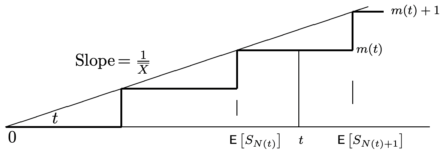
We derive an upper bound on \(\mathrm{E}\left[S_{N(t)+1}\right]\) in the next section. First, however, as a santity check, consider Figure 4.12 which illustrates \ref{4.35} for the case where each \(X_{n}\) is a deterministic rv where \(X_{n}=\bar{X}\) with probability 1.

Figure 4.12: Illustration of \ref{4.34} for the special case where \(X\) is deterministic. Note that \(m(t)\), as a function of \(t\), is then the illustrated staircase function. On each increment of \(t\) by \(\bar{X}\), \(m(t)\) increases by one. Then \(m(t)+1\) and \(\mathrm{E}\left[S_{N(t)+1}\right]\) are two sides of a right triangle of slope \(1 / \bar{X}\), yielding (4.34).

It might be puzzling why we used \(N(t)+1\) rather than \(N(t)\) as a stopping trial for the epochs \(\left\{S_{i} ; i \geq 1\right\}\) in this application of Wald’s equality. To understand this, assume for example that \(N(t)=n\). When an observer sees the sample values of \(S_{1}, \ldots, S_{n}\), with \(S_{n}<t\), the observer typically cannot tell (on the basis of \(S_{1}, \ldots, S_{n}\) alone) whether any other arrivals will occur in the interval \(\left(S_{n}, t\right]\). In other words, \(N(t)=n\) implies that \(S_{n} \leq t\), but \(S_{n}<t\) does not imply that \(N(t)=n\). On the other hand, still assuming \(N(t)=n\), an observer seeing \(S_{1}, \ldots, S_{n+1}\) knows that \(N(t)=n\).

Any stopping trial (for an arbitrary sequence of rv’s \(\left\{S_{n} ; n \geq 1\right\}\)) can be viewed as an experiment where an observer views sample values \(s_{1}, s_{2}, \ldots\), in turn until the stopping rule is satisfied. The stopping rule does not permit either looking ahead or going back to change an earlier decision. Thus the rule: stop at \(N(t)+1\) (for the renewal epochs \(\left\{S_{n} ; n \geq 1\right\}\)) means stop at the first sample value \(\boldsymbol{S}_{i}\) that exceeds \(t\). Stopping at the final sample value \(s_{n} \leq t\) is not necessarily possible without looking ahead to the following sample value.

Stopping trials, embedded renewals, and G/G/1 queues

The above definition of a stopping trial is quite restrictive in that it refers only to a single sequence of rv’s. In many queueing situations, for example, there is both a sequence of interarrival times \(\left\{X_{i} ; i \geq 1\right\}\) and a sequence of service times \(\left\{V_{i} ; i \geq 0\right\}\). Here \(X_{i}\) is the interarrival interval between customer \(i-1\) and \(i\), where an initial customer 0 is assumed to arrive at time 0, and \(X_{1}\) is the arrival time for customer 1. The service time of customer 0 is then \(V_{0}\) and each \(V_{i}\), \(i>0\) is the service time of the corresponding ordinary customer. Customer number 0 is not ordinary in the sense that it arrives at the fixed time 0 and is not counted in the arrival counting process \(\{N(t) ; t>0\}\).

Example 4.5.3 (G/G/1 queues:).

Consider a G/G/1 queue (the single server case of the G/G/m queue described in Example 4.1.2). We assume that the customers are served in First-Come-First-Served (FCFS) order.¹² Both the interarrival intervals \(\left\{X_{i} ; i \geq 1\right\}\) and the service times \(\left\{V_{i} ; i \geq 0\right\}\) are assumed to be IID and the service times are assumed to be independent of the interarrival intervals. Figure 4.13 illustrates a sample path for these arrivals and departures.

Customer 2 arrives at \(s_{2}=x_{1}+x_{2}\). For the case shown above, this is before customer 1 departs at \(v_{0}+v_{1}\). Thus, customer 2’s wait in queue is \(w_{2}^{q}=v_{0}+v_{1}-x_{1}-x_{2}\). As illustrated above, \(x_{2}+w_{2}^{q}\) is also equal to customer 1’s system time, so \(w_{2}^{q}=w_{1}^{q}+v_{1}-x_{2}\). Customer 3 arrives when the system is empty, so it enters service immediately with no wait in queue, i.e., \(w_{3}^{q}=0\).

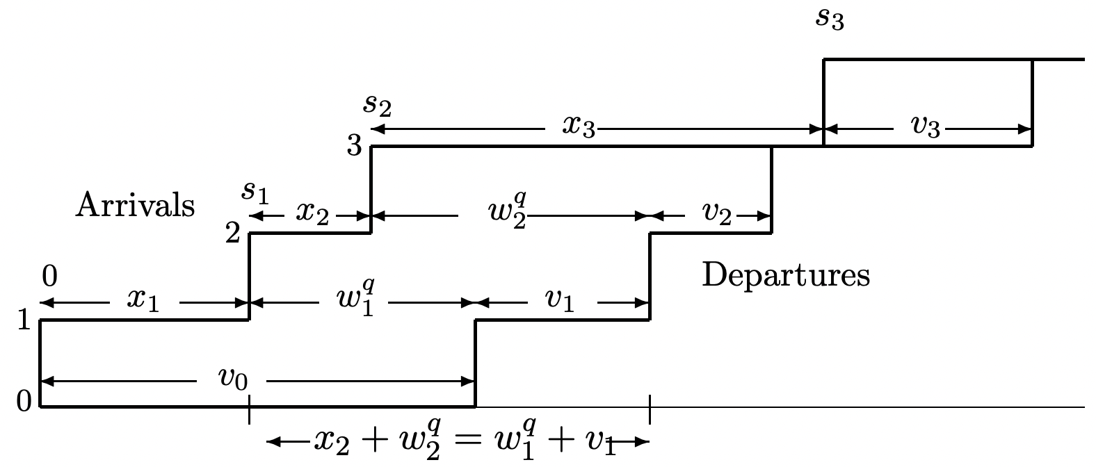
The figure illustrates a sample path for which \(X_{1}<V_{0}\), so arrival number 1 waits in queue for \(W_{1}^{q}=V_{0}-X_{1}\). If \(X_{1} \geq V_{0}\), on the other hand, then customer one enters service immediately, i.e., customer one ‘sees an empty system.’ In general, then W_1^q=\max \left(V_{0}-X_{1}, 0\right). In the same way, as illustrated in the figure, if \(W_{1}^{q}>0\), then customer 2 waits for \(W_{1}^{q}+V_{1}-X_{2}\) if positive and 0 otherwise. This same formula works if \(W_{1}^{q}=0\), so \(W_{2}^{q}=\max \left(W_{1}^{q}+V_{1}-X_{2}, 0\right)\). In general, it can be seen that

\[W_{i}^{q}=\max \left(W_{i-1}^{q}+V_{i-1}-X_{i}, 0\right)\label{4.37} \]

This equation will be analyzed further in Section 7.2 where we are interested in queueing delay and system delay. Here our objectives are simpler, since we only want to show that the subsequence of customer arrivals \(i\) for which the event \(\left\{W_{i}^{q}=0\right\}\) is satisfied form the renewal epochs of a renewal process. To do this, first observe from \ref{4.37} (using induction if desired) that \(W_{i}^{q}\) is a function of \(\left(X_{1}, \ldots, X_{i}\right)\) and \(\left(V_{0}, \ldots, V_{i-1}\right)\). Thus, if we let \(J\) be the smallest \(i>0\) for which \(W_{i}^{q}=0\), then \(\mathbb{I}_{J=i}\) is a function of \(\left(X_{1}, \ldots, X_{i}\right)\) and \(\left(V_{0}, \ldots, V_{i-1}\right)\).

We now interrupt the discussion of G/G/1 queues with the following generalization of the definition of a stopping trial.

Definition 4.5.2 (Generalized stopping trials).

A generalized stopping trial \(J\) for a sequence of pairs of rv’s \(\left(X_{1}, V_{1}\right),\left(X_{2}, V_{2}\right) \ldots\), is a positive integer-valued rv such that, for each \(n \geq 1\), the indicator rv \(\mathbb{I}_{\{J=n\}}\) is a function of \(X_{1}, V_{1}, X_{2}, V_{2}, \ldots, X_{n}, V_{n}\).

Wald’s equality can be trivially generalized for these generalized stopping trials.

Theorem 4.5.2 (Generalized Wald's equality).

Let \(\left\{\left(X_{n}, V_{n}\right) ; n \geq 1\right\}\) be a sequence of pairs of rv’s, where each pair is independent and identically distributed (IID) to all other pairs. Assume that each \(X_{i}\) has finite mean \(\bar{X}\). If \(J\) is a stopping trial for \(\left\{\left(X_{n}, V_{n}\right) ; n \geq 1\right\}\) and if \(\mathrm{E}[J]<\infty\), then the sum \(S_{J}=X_{1}+X_{2}+\cdots+X_{J}\) satisfies

\[\mathrm{E}\left[S_{J}\right]=\bar{X} \mathrm{E}[J]\label{4.38} \]

Proof

The proof of this will be omitted, since it is the same as the proof of Theorem 4.5.1. In fact, the definition of stopping trials could be further generalized by replacing the rv’s \(V_{i}\) by vector rv’s or by a random number of rv’s , and Wald’s equality would still hold.¹³

For the example of the G/G/1 queue, we take the sequence of pairs to be \(\left\{\left(X_{1}, V_{0}\right),\left(X_{2}, V_{1}\right), \ldots,\right\}\). Then \(\left\{\left(X_{n}, V_{n-1} ; n \geq 1\right\}\right.\) satisfies the conditions of Theorem 4.5.2 (assuming that \(\mathrm{E}\left[X_{i}\right]<\infty\). Let \(J\) be the generalized stopping rule specifying the number of the first arrival to find an empty queue. Then the theorem relates \(\mathrm{E}\left[S_{J}\right]\), the expected time \(t>0\) until the first arrival to see an empty queue, and \(\mathrm{E}[J]\), the expected number of arrivals until seeing an empty queue.

It is important here, as in many applications, to avoid the confusion created by viewing \(J\) as a stopping time. We have seen that \(J\) is the number of the first customer to see an empty queue, and \(S_{J}\) is the time until that customer arrives.

There is a further possible timing confusion about whether a customer’s service time is determined when the customer arrives or when it completes service. This makes no difference, since the ordered sequence of pairs is well-defined and satisfies the appropriate IID condition for using the Wald equality.

As is often the case with Wald’s equality, it is not obvious how to compute either quantity in (4.38), but it is nice to know that they are so simply related. It is also interesting to see that, although successive pairs \(\left(X_{i}, V_{i}\right)\) are assumed independent, it is not necessary for \(X_{i}\) and \(V_{i}\) to be independent. This lack of independence does not occur for the G/G/1 (or G/G/m) queue, but can be useful in situations such as packet networks where the interarrival time between two packets at a given node can depend on the service time (the length) of the first packet if both packets are coming from the same node.

Perhaps a more important aspect of viewing the first renewal for the G/G/1 queue as a stopping trial is the ability to show that successive renewals are in fact IID. Let \(X_{2,1}, X_{2,2}, \ldots\) be the interarrival times following \(J\), the first arrival to see an empty queue. Conditioning on \(J=j\), we have \(X_{2,1}=X_{j+1}, X_{2,2}=X_{j+2}, \ldots,\). Thus \(\left\{X_{2, k} ; k \geq 1\right\}\) is an IID sequence with the original interarrival distribution. Similarly \(\left\{\left(X_{2, k}, V_{2, k}\right) ; k \geq 1\right\}\) is a sequence of IID pairs with the original distribution. This is valid for all sample values \(j\) of the stopping trial \(J\). Thus \(\left\{\left(X_{2, k}, V_{2, k}\right) ; k \geq 1\right\}\) is statistically independent of \(J\) and \(\left(X_{i}, V_{i}\right) ; 1 \leq i \leq J\).

The argument above can be repeated for subsequent arrivals to an empty system, so we have shown that successive arrivals to an empty system actually form a renewal process.¹⁴

One can define many different stopping rules for queues, such as the first trial at which a given number of customers are in the queue. Wald’s equality can be applied to any such stopping rule, but much more is required for the stopping trial to also form a renewal point. At the first time when n customers are in the system, the subsequent departure times depend partly on the old service times and partly on the new arrival and service times, so the required independence for a renewal point does not exist. Stopping rules are helpful in understanding embedded renewal points, but are by no means equivalent to embedded renewal points.

Finally, nothing in the argument above for the G/G/1 queue made any use of the FCFS service discipline. One can use any service discipline for which the choice of which customer to serve at a given time \(t\) is based solely on the arrival and service times of customers in the system by time \(t\). In fact, if the server is never idle when customers are in the system, the renewal epochs will not depend on the service descipline. It is also possible to extend these arguments to the G/G/m queue, although the service discipline can affect the renewal points in this case.

Little’s theorem

Little’s theorem is an important queueing result stating that the expected number of customers in a queueing system is equal to the product of the arrival rate and the expected time each customer waits in the system. This result is true under very general conditions; we use the G/G/1 queue with FCFS service as a specific example, but the reason for the greater generality will be clear as we proceed. Note that the theorem does not tell us how to find either the expected number or expected wait; it only says that if one can be found, the other can also be found.

The figure also shows the sample values \(s_{1}^{r}\) and \(s_{2}^{r}\) of the first two arrivals that see an empty system (recall from Section 4.5.3 that the subsequence of arrivals that see an empty system forms a renewal process.)

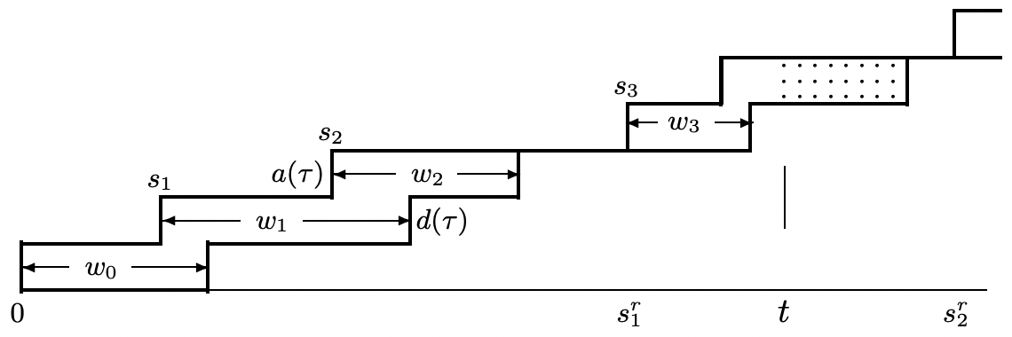
Figure 4.14 illustrates a sample path for a G/G/1 queue with FCFS service. It illustrates a sample path \(a(t)\) for the arrival process \(A(t)=N(t)+1\), i.e., the number of customer arrivals in \([0, t]\), specifically including customer number 0 arriving at \(t=0\). Similarly, it illustrates the departure process \(D(t)\), which is the number of departures up to time \(t\), again including customer 0. The difference, \(L(t)=A(t)-D(t)\), is then the number in the system at time \(t\).

Recall from Section 4.5.3 that the subsequence of customer arrivals for \(t>0\) that see an empty system form a renewal process. Actually, we showed a little more than that. Not only are the inter-renewal intervals, \(X_{i}^{r}=S_{i}^{r}-S_{i-1}^{r}\) IID, but the number of customer arrivals in each inter-renewal interval are IID, and the interarrival intervals and service times between inter-renewal intervals are IID. The sample values, \(s_{1}^{r}\) and \(s_{2}^{r}\) of the first two renewal epochs are shown in the figure.

The essence of Little’s theorem can be seen by observing that \(\int_{0}^{S_{1}^{r}} L(\tau) d \tau\) in the figure is the area between the upper and lower step functions, integrated out to the first time that the two step functions become equal (i.e., the system becomes empty). For the sample value in the figure, this integral is equal to \(w_{0}+w_{1}+w_{2}\). In terms of the rv’s,

\[\int_{0}^{S_{1}^{r}} L(\tau) d \tau=\sum_{i=0}^{N\left(S_{1}^{r}\right)-1} W_{i}\label{4.39} \]

The same relationship exists in each inter-renewal interval, and in particular we can define \(L_{n}\) for each \(n \geq 1\) as

\[L_{n}=\int_{S_{n-1}^{r}}^{S_{n}^{r}} L(\tau) d \tau=\sum_{i=N\left(S_{n-1}^{r}\right)}^{N\left(S_{n}^{r}\right)-1} W_{i}\label{4.40} \]

The interpretation of this is far simpler than the notation. The arrival step function and the departure step function in Figure 4.14 are separated whenever there are customers in the system (the system is busy) and are equal whenever the system is empty. Renewals occur when the system goes from empty to busy, so the \(n\)th renewal is at the beginning of the \(n\)th busy period. Then \(L_{n}\) is the area of the region between the two step functions over the \(n\)th busy period. By simple geometry, this area is also the sum of the customer waiting times over that busy period. Finally, since the interarrival intervals and service times in each busy period are IID with respect to those in each other busy period, the sequence \(L_{1}, L_{2}, \ldots\), is a sequence of IID rv’s.

The function \(L(\tau)\) has the same behavior as a renewal reward function, but it is slightly more general, being a function of more than the age and duration of the renewal counting process \(\left\{N^{r}(t) ; t>0\right\}\) at \(t=\tau\). However the fact that \(\left\{L_{n} ; n \geq 1\right\}\) is an IID sequence lets us use the same methodology to treat \(L(\tau)\) as was used earlier to treat renewal-reward functions. We now state and prove Little’s theorem. The proof is almost the same as that of Theorem 4.4.1, so we will not dwell on it.

Theorem 4.5.3 (Little).

For a FCFS G/G/1 queue in which the expected inter-renewal interval is finite, the limiting time-average number of customers in the system is equal, with probability 1, to a constant denoted as \(\overline{L}\). The sample-path-average waiting time per customer is also equal, with probability 1, to a constant denoted as \(\overline{W}\). Finally \(\overline{L}=\lambda \overline{W}\) where \(\lambda\) is the customer arrival rate, i.e., the reciprocal of the expected interarrival time.

Proof

Note that for any \(t>0\), \(\int_{0}^{t}(L(\tau) d \tau\) can be expressed as the sum over the busy periods completed before \(t\) plus a residual term involving the busy period including \(t\). The residual term can be upper bounded by the integral over that complete busy period. Using this with (4.40), we have

\[\sum_{n=1}^{N^{r}(t)} \mathrm{L}_{n} \leq \int_{\tau=0}^{t} L(\tau) d \tau \leq \sum_{i=0}^{N(t)} W_{i} \leq \sum_{n=1}^{N^{r}(t)+1} \mathrm{~L}_{n}\label{4.41} \]

Assuming that the expected inter-renewal interval, \(\mathrm{E}\left[X^{r}\right]\), is finite, we can divide both sides of \ref{4.41} by \(t\) and go to the limit \(t \rightarrow \infty\). From the same argument as in Theorem 4.4.1,

\[\lim _{t \rightarrow \infty} \frac{\sum_{i=0}^{N(t)} W_{i}}{t}=\lim _{t \rightarrow \infty} \frac{\int_{\tau=0}^{t} L(\tau) d \tau}{t}=\frac{\mathrm{E}\left[\mathrm{L}_{n}\right]}{\mathrm{E}\left[X^{r}\right]} \quad \text { with probability } 1\label{4.42} \]

The equality on the right shows that the limiting time average of \(L(\tau)\) exists with probability 1 and is equal to \(\overline{L}=\mathrm{E}\left[L_{n}\right] / \mathrm{E}\left[X^{r}\right]\). The quantity on the left of \ref{4.42} can now be broken up as waiting time per customer multiplied by number of customers per unit time, i.e.,

\[\lim _{t \rightarrow \infty} \frac{\sum_{i=0}^{N(t)} W_{i}}{t}=\lim _{t \rightarrow \infty} \frac{\sum_{i=0}^{N(t)} W_{i}}{N(t)} \lim _{t \rightarrow \infty} \frac{N(t)}{t}\label{4.43} \]

From (4.42), the limit on the left side of \ref{4.43} exists (and equals \(\overline{L}\)) with probability 1. The second limit on the right also exists with probability 1 by the strong law for renewal processes, applied to \(\{N(t) ; t>0\}\). This limit is called the arrival rate \(\lambda\), and is equal to the reciprocal of the mean interarrival interval for \(\{N(t)\}\). Since these two limits exist with probability 1, the first limit on the right, which is the sample-path-average waiting time per customer, denoted \(\overline{W}\), also exists with probability 1.

Reviewing this proof and the development of the G/G/1 queue before the theorem, we see that there was a simple idea, expressed by (4.39), combined with a lot of notational complexity due to the fact that we were dealing with both an arrival counting process \(\{N(t) ; t>0\}\) and an embedded renewal counting process \(\left\{N^{r}(t) ; t>0\right\}\). The difficult thing, mathematically, was showing that \(\left\{N^{r}(t) ; t>0\right\}\) is actually a renewal process and showing that the \(L_{n}\) are IID, and this was where we needed to understand stopping rules.

Recall that we assumed earlier that customers departed from the queue in the same order in which they arrived. From Figure 4.15, however, it is clear that FCFS order is not required for the argument. Thus the theorem generalizes to systems with multiple servers and arbitrary service disciplines in which customers do not follow FCFS order. In fact, all that the argument requires is that the system has renewals (which are IID by definition of a renewal) and that the inter-renewal interval is finite with probability 1.

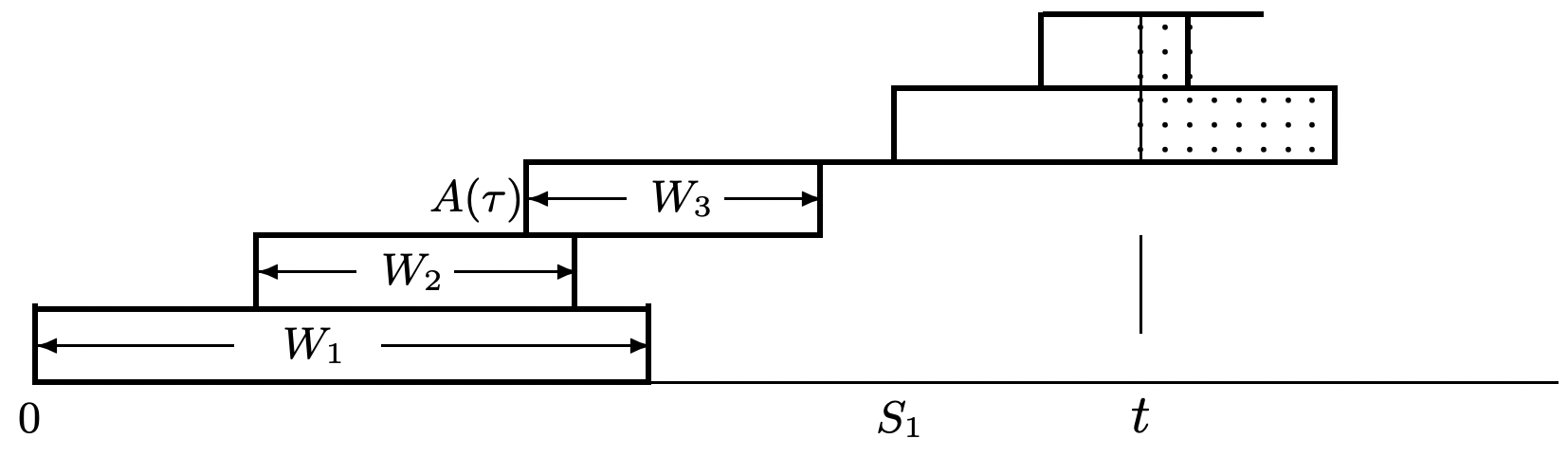Figure 4.15: Arrivals and departures in a non-FCFS systems. The server, for example, could work simultaneously (at a reduced rate) on all customers in the system, and thus complete service for customers with small service needs before completing earlier arrivals with greater service needs. Note that the jagged right edge of the diagram does not represent number of deparatures, but this is not essential for the argument.

For example, if higher priority is given to customers with small service times, then it is not hard to see that the average number of customers in the system and the average waiting time per customer will be decreased. However, if the server is always busy when there is work to be done, it can be seen that the renewal times are unaffected. Service discipines will be discussed further in Section 5.6.

The same argument as in Little’s theorem can be used to relate the average number of customers in a single server queue (not counting service) to the average wait in the queue (not counting service). Renewals still occur on arrivals to an empty system, and the integral of customers in queue over a busy period is still equal to the sum of the queue waiting times. Let \(L^{q}(t)\) be the number in the queue at time \(t\) and let \(\bar{L}^{q}=\lim _{t \rightarrow \infty}(1 / t) \int_{0}^{t} L^{q}(\tau) d \tau\) be the time-average queue wait. Letting \(\overline{W}^{q}\) be the sample-path-average waiting time in queue,

\[\overline{L}^{q}=\lambda \overline{W}^{q} \label{4.44} \]

The same argument can also be applied to the service facility of a single server queue. The time-average of the number of customers in the server is just the fraction of time that the server is busy. Denoting this fraction by \(\rho\) and the expected service time by \(\overline{V}\), we get

\[\rho=\lambda \overline{V}\label{4.45} \]

Expected queueing time for an M/G/1 queue

For our last example of the use of renewal-reward processes, we consider the expected queueing time in an M/G/1 queue. We again assume that an arrival to an empty system occurs at time 0 and renewals occur on subsequent arrivals to an empty system. At any given time \(t\), let \(L^{q}(t)\) be the number of customers in the queue (not counting the customer in service, if any) and let \(R(t)\) be the residual life of the customer in service. If no customer is in service, \(R(t)=0\), and otherwise \(R(t)\) is the remaining time until the current service is completed. Let \(U(t)\) be the waiting time in queue that would be experienced by a customer arriving at time \(t\). This is often called the unfinished work in the queueing literature and represents the delay until all the customers currently in the system complete service. Thus the rv \(U(t)\) is equal to \(R(t)\), the residual life of the customer in service, plus the service times of each of the \(L^{q}(t)\) customers currently waiting in the queue.

\[U(t)=\sum_{i=1}^{L^{q}(t)} V_{N(t)-i}+R(t),\label{4.46} \]

where \(N(t)-i\) is the customer number of the \(i\)th customer in the queue at time \(t\). Since \(L^{q}(t)\) is a function only of the interarrival times in \((0, t)\) and the service times of the customers that have already been served, we see that for each sample value \(L^{q}(t)=\ell\), the rv’s \(\widetilde{V}_{1}, \ldots, \widetilde{V}_{\ell}\) each have the service time distribution \(\mathrm{F}_{V}\). Thus, taking expected values,

\[\mathrm{E}[U(t)]=\mathrm{E}\left[L^{q}(t)\right] \mathrm{E}[V]+\mathrm{E}[R(t)].\label{4.47} \]

Figure 4.16 illustrates how to find the time-average of \(R(t)\). Viewing \(R(t)\) as a reward

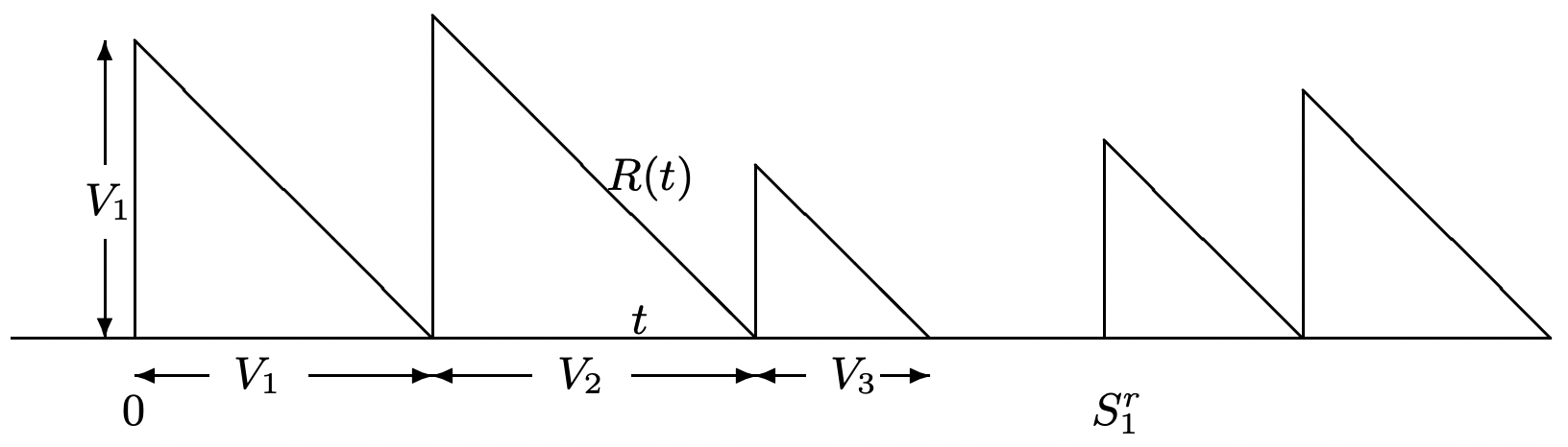Figure 4.16: Sample value of the residual life function of customers in service.

function, we can find the accumulated reward up to time t as the sum of triangular areas.

First, consider \(\int R(\tau) d \tau\) from 0 to \(S_{N^{r}(t)}^{r}\), i.e., the accumulated reward up to the final renewal epoch in \([o, t] t\). Note that \(S_{N^{r}(t)}^{r}\) is not only a renewal epoch for the renewal process, but also an arrival epoch for the arrival process; in particular, it is the \(N\left(S_{N^{r}(t)}^{r}\right) \text { th }\) arrival epoch, and the \(N\left(S_{N^{r}(t)}^{r}\right)-1\) earlier arrivals are the customers that have received service up to time \(S_{N^{r}(t)}^{r}\). Thus,

\(\int_{0}^{S_{N^{r}(t)}^{r}} R(\tau) d \tau=\sum_{i=0}^{N\left(S_{N^{r}(t)}^{r}\right)-1} \frac{V_{i}^{2}}{2} \leq \sum_{i=0}^{N(t)} \frac{V_{i}^{2}}{2}.\)

We can similarly upper bound the term on the right above by \(\int_{0}^{S_{N^{r}(t)+1}^{r}} R(\tau) d \tau\). We also know (from going through virtually the same argument several times) that \((1 / t) \int_{\tau=0}^{t} R(\tau) d \tau\) will approach a limit¹⁵ with probability 1 as \(t \rightarrow \infty\), and that the limit will be unchanged if \(t\) is replaced with \(S_{N^{r}(t)}^{r}\) or \(S_{N^{r}(t)+1}^{r}\). Thus, taking \(\lambda\) as the arrival rate,

\(\lim _{t \rightarrow \infty} \frac{\int_{0}^{t} R(\tau) d \tau}{t}=\lim _{t \rightarrow \infty} \frac{\sum_{i=1}^{A(t)} V_{i}^{2}}{2 A(t)} \frac{A(t)}{t}=\frac{\lambda \mathrm{E}\left[V^{2}\right]}{2}\quad\text{WP1}\)

We will see in the next section that the time average above can be replaced with a limiting ensemble-average, so that

\[\lim _{t \rightarrow \infty} \mathrm{E}[R(t)]=\frac{\lambda \mathrm{E}\left[V^{2}\right]}{2}.\label{4.48} \]

The next section also shows that there is a limiting ensemble-average form of (4.44), showing that \(\lim _{t \rightarrow \infty} \mathrm{E}\left[L^{q}(t)\right]=\lambda \overline{W}^{q}\). Substituting this plus \ref{4.48} into (4.47), we get

\[\lim _{t \rightarrow \infty} \mathrm{E}[U(t)]=\lambda \mathrm{E}[V] \overline{W}^{q}+\frac{\lambda \mathrm{E}\left[V^{2}\right]}{2}.\label{4.49} \]

Thus \(\mathrm{E}[U(t)]\) is asymptotically independent of \(t\). It is now important to distinguish between \(\mathrm{E}[U(t)]\) and \(\overline{W}^{q}\). The first is the expected unfinished work at time \(t\), which is the queueing delay that a customer would incur by arriving at \(t\); the second is the sample-path-average expected queueing delay. For Poisson arrivals, the probability of an arrival in \((t, t+\delta]\) is independent of all earlier arrivals and service times, so it is independent of \(U(t)\) ¹⁶. Thus, in the limit \(t \rightarrow \infty\), each arrival faces an expected delay \(\lim _{t \rightarrow \infty} \mathrm{E}[U(t)]\), so \(\lim _{t \rightarrow \infty} \mathrm{E}[U(t)]\) must be equal to \(\overline{W}^{q}\). Substituting this into (4.49), we obtain the celebrated PollaczekKhinchin formula,

\[\overline{W}^{q}=\frac{\lambda \mathrm{E}\left[V^{2}\right]}{2(1-\lambda \mathrm{E}[V])}.\label{4.50} \]

This queueing delay has some of the peculiar features of residual life, and in particular, if \(\mathrm{E}\left[V^{2}\right]=\infty\), the limiting expected queueing delay is infinite even when the expected service time is less than the expected interarrival interval.

In trying to visualize why the queueing delay is so large when \(\mathrm{E}\left[V^{2}\right]\) is large, note that while a particularly long service is taking place, numerous arrivals are coming into the system, and all are being delayed by this single long service. In other words, the number of new customers held up by a long service is proportional to the length of the service, and the amount each of them are held up is also proportional to the length of the service. This visualization is rather crude, but does serve to explain the second moment of \(V\) in (4.50). This phenomenon is sometimes called the “slow truck effect” because of the pile up of cars behind a slow truck on a single lane road.

For a G/G/1 queue, \ref{4.49} is still valid, but arrival times are no longer independent of \(U(t)\), so that typically \(\mathrm{E}[U(t)] \neq \overline{W}^{q}\). As an example, suppose that the service time is uniformly distributed between \(1-\epsilon\) and \(1+\epsilon\) and that the interarrival interval is uniformly distributed between \(2-\epsilon\) and \(2+\epsilon\). Assuming that \(\epsilon<1 / 2\), the system has no queueing and \(\overline{W}^{q}=0\). On the other hand, for small \(\epsilon\), \(\lim _{t \rightarrow \infty} \mathrm{E}[U(t)] \sim 1 / 4\) (i.e., the server is busy half the time with unfinished work ranging from 0 to 1).

---

⁸For example, poker players do not take kindly to a player who attempts to withdraw his bet when someone else wins the hand. Similarly, a statistician gathering data on product failures should not respond to a failure by then recording an earlier trial as a stopping time, thus not recording the failure.

⁹Stopping trials are more often called stopping times or optional stopping times in the literature. In our first major application of a stopping trial, however, the stopping trial is the first trial \(n\) at which a renewal epoch \(S_{n}\) exceeds a given time \(t\). Viewing this trial as a time generates considerable confusion.

¹⁰This can be quite confusing initially, since (as seen in the example of Figure 4.11) \(X_{n}\) is not necessarily independent of the event \(\{J=n\}\), nor of \(\{J=n+1\}\), etc. In other words, given that stopping has not occurred before trial \(n\), then \(X_{n}\) can have a great deal to do with the trial at which stopping occurs. However, as shown above, \(X_{n}\) has nothing to do with whether \(\{J<n\}\) or \(\{J \geq n\}\).

¹¹This will be shown when we view this example as a birth-death Markov chain in Chapter 5.

¹²For single server queues, this is sometimes referred to as First-In-First-Out (FIFO) service.

¹³In fact, \(J\) is sometimes defined to be a stopping rule if \(\mathbb{I}_{\{J \geq n\}}\) is independent of \(X_{n}, X_{n+1}, \ldots\) for each \(n\). This makes it easy to prove Wald’s equality, but quite hard to see when the definition holds, especially since \(\mathbb{I}_{\{J=n\}}\), for example, is typically dependent on \(X_{n}\) (see footnote 7).

¹⁴Confession by author: For about 15 years, I mistakenly believed that it was obvious that arrivals to an empty system in a G/G/m queue form a renewal process. Thus I can not expect readers to be excited about the above proof. However, it is a nice example of how to use stopping times to see otherwise murky points clearly.

¹⁵In fact, one could simply take the limit without bringing in the renewal process, since it is clear by now that the renewal process justifies the limit with probability 1.

¹⁶This is often called the PASTA property, standing for Poisson arrivals see time-averages. This holds with great generality, requiring only that time-averages exist and that the parameters of interest at a given time \(t\) are independent of future arrivals. At the same time, this property is somewhat vague, so it should be used to help the intuition rather than to prove theorems.