4.4: Renewal-Reward Processes and Time-Averages

There are many situations in which, along with a renewal counting process \(\{N(t) ; t>0\}\), there is another randomly varying function of time, called a reward function \(\{R(t) ; t>0\}\). \(R(t)\) models a rate at which the process is accumulating a reward. We shall illustrate many examples of such processes and see that a “reward” could also be a cost or any randomly varying quantity of interest. The important restriction on these reward functions is that \(R(t)\) at a given \(t\) depends only on the location of \(t\) within the inter-renewal interval containing \(t\) and perhaps other random variables local to that interval. Before defining this precisely, we start with several examples.

Example 4.4.4 (Time-average residual life)

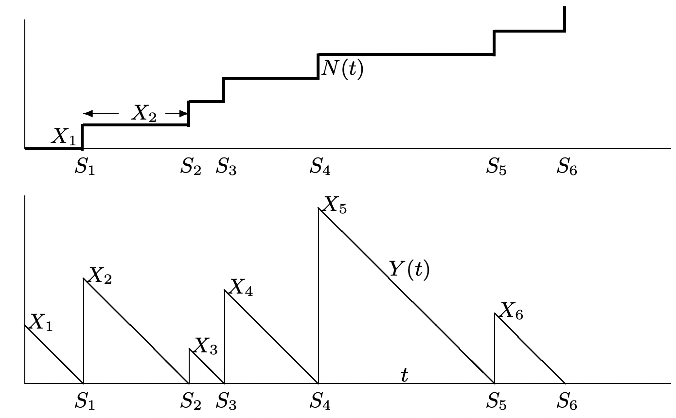
For a renewal counting process \(\{N(t), t>0\}\), let \(Y(t)\) be the residual life at time \(t\). The residual life is defined as the interval from \(t\) until the next renewal epoch, i.e., as \(S_{N(t)+1}-t\). For example, if we arrive at a bus stop at time \(t\) and buses arrive according to a renewal process, \(Y(t)\) is the time we have to wait for a bus to arrive (see Figure 4.5). We interpret \(\{Y(t) ; t \geq 0\}\) as a reward function. The timeaverage of \(Y(t)\), over the interval \((0, t]\), is given by⁵ \((1 / t) \int_{0}^{t} Y(\tau) d \tau\). We are interested in the limit of this average as \(t \rightarrow \infty\) (assuming that it exists in some sense). Figure 4.5 illustrates a sample function of a renewal counting process \(\{N(t) ; t>0\}\) and shows the residual life \(Y(t)\) for that sample function. Note that, for a given sample function \(\{Y(t)=y(t)\}\), the integral \(\int_{0}^{t} y(\tau) d \tau\) is simply a sum of isosceles right triangles, with part of a final triangle at the end. Thus it can be expressed as

\(\int_{0}^{t} y(\tau) d \tau=\frac{1}{2} \sum_{i=1}^{n(t)} x_{i}^{2}+\int_{\tau=s_{n(t)}}^{t} y(\tau) d \tau\)

where \(\left\{x_{i} ; 0<i<\infty\right\}\) is the set of sample values for the inter-renewal intervals.

Since this relationship holds for every sample point, we see that the random variable \(\int_{0}^{t} Y(\tau) d \tau\) can be expressed in terms of the inter-renewal random variables \(X_{n}\) as

\(\int_{\tau=0}^{t} Y(\tau) d \tau=\frac{1}{2} \sum_{n=1}^{N(t)} X_{n}^{2}+\int_{\tau=S_{N(t)}}^{t} Y(\tau) d \tau\)

Figure 4.5: Residual life at time \(t\). For any given sample function of the renewal process, the sample function of residual life decreases linearly with a slope of −1 from the beginning to the end of each inter-renewal interval.

Although the final term above can be easily evaluated for a given \(S_{N(t)}(t)\), it is more convenient to use the following bound:

\[\frac{1}{2 t} \sum_{n=1}^{N(t)} X_{n}^{2} \leq \frac{1}{t} \int_{\tau=0}^{t} Y(\tau) d \tau \leq \frac{1}{2 t} \sum_{n=1}^{N(t)+1} X_{n}^{2}\label{4.11} \]

The term on the left can now be evaluated in the limit \(t \rightarrow \infty\) (for all sample functions except a set of probability zero) as follows:

\[\lim _{t \rightarrow \infty} \frac{\sum_{n=1}^{N(t)} X_{n}^{2}}{2 t}=\lim _{t \rightarrow \infty} \frac{\sum_{n=1}^{N(t)} X_{n}^{2}}{N(t)} \frac{N(t)}{2 t}\label{4.12} \]

Consider each term on the right side of \ref{4.12} separately. For the first term, recall that \(\lim _{t \rightarrow 0} N(t)=\infty\) with probability 1. Thus as \(t \rightarrow \infty\), \(\sum_{n=1}^{N(t)} X_{n}^{2} / N(t)\) goes through the same set of values as \(\sum_{n=1}^{k} X_{n}^{2} / k\) as \(k \rightarrow \infty\). Thus, using the SLLN,

\(\lim _{t \rightarrow \infty} \frac{\sum_{n=1}^{N(t)} X_{n}^{2}}{N(t)}=\lim _{k \rightarrow \infty} \frac{\sum_{n=1}^{k} X_{n}^{2}}{k}=\mathrm{E}\left[X^{2}\right] \quad \text{WP1}\),

The second term on the right side of \ref{4.12} is simply \(N(t) / 2 t\). By the strong law for renewal processes, \(\lim _{t \rightarrow \infty} N(t) / 2 t=1 /(2 \mathrm{E}[X])\) WP1. Thus both limits exist WP1 and

\[\lim _{t \rightarrow \infty} \frac{\sum_{n=1}^{N(t)} X_{n}^{2}}{2 t}=\frac{\mathrm{E}\left[X^{2}\right]}{2 \mathrm{E}[X]}\quad \text{WP1}\label{4.13} \]

The right hand term of \ref{4.11} is handled almost the same way:

\[\lim _{t \rightarrow \infty} \frac{\sum_{n=1}^{N(t)+1} X_{n}^{2}}{2 t}=\lim _{t \rightarrow \infty} \frac{\sum_{n=1}^{N(t)+1} X_{n}^{2}}{N(t)+1} \frac{N(t)+1}{N(t)} \frac{N(t)}{2 t}=\frac{\mathrm{E}\left[X^{2}\right]}{2 \mathrm{E}[X]}\label{4.14} \]

Combining these two results, we see that, with probability 1, the time-average residual life is given by

\[\lim _{t \rightarrow \infty} \frac{\int_{\tau=0}^{t} Y(\tau) d \tau}{t}=\frac{\mathrm{E}\left[X^{2}\right]}{2 \mathrm{E}[X]}\label{4.15} \]

Note that this time-average depends on the second moment of \(X\); this is \(\bar{X}^{2}+\sigma^{2} \geq \bar{X}^{2}\), so the time-average residual life is at least half the expected inter-renewal interval (which is not surprising). On the other hand, the second moment of \(X\) can be arbitrarily large (even infinite) for any given value of \(\mathrm{E}[X]\), so that the time-average residual life can be arbitrarily large relative to \(\mathrm{E}[X]\). This can be explained intuitively by observing that large interrenewal intervals are weighted more heavily in this time-average than small inter-renewal intervals.

Example 4.4.2

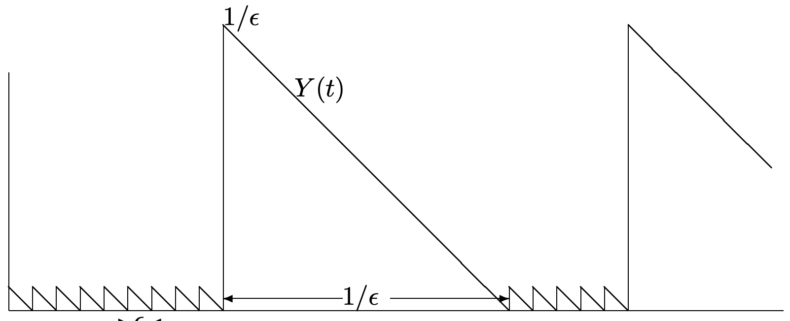
As an example of the effect of improbable but large inter-renewal intervals, let \(X\) take on the value \(\epsilon\) with probability \(1-\epsilon\) and value \(1 / \epsilon\) with probability \(\epsilon\). Then, for small \(\epsilon\), \(\mathrm{E}[X] \sim 1, \mathrm{E}\left[X^{2}\right] \sim 1 / \epsilon\), and the time average residual life is approximately \(1 /(2 \epsilon)\) (see Figure 4.6).

Figure 4.6: Average Residual life is dominated by large interarrival intervals. Each large interval has duration \(1 / \epsilon\), and the expected aggregate duration between successive large intervals is \(1-\epsilon\)

Example 4.4.3. (timer-average Age)

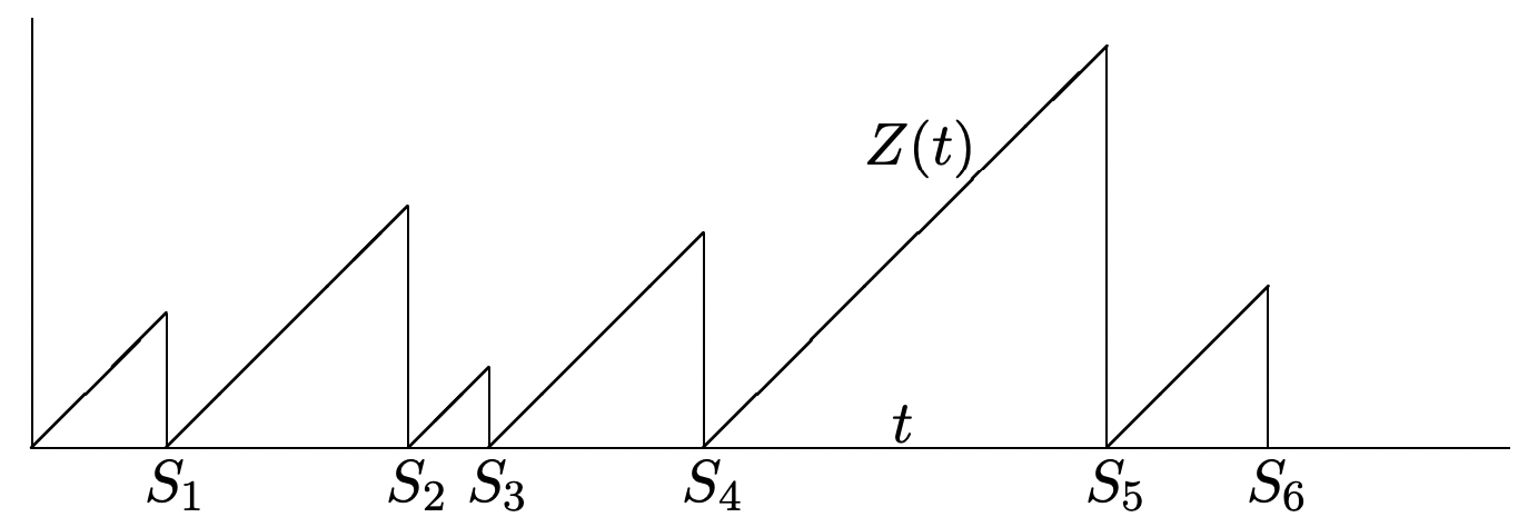
Let \(Z(t)\) be the age of a renewal process at time \(t\) where age is defined as the interval from the most recent arrival before (or at) \(t\) until \(t\), i.e., \(Z(t)=t-S_{N(t)}\). By convention, if no arrivals have occurred by time \(t\), we take the age to be \(t\) (i.e., in this case, \(N(t)=0\) and we take \(S_{0}\) to be 0).

As seen in Figure 4.16, the age process, for a given sample function of the renewal process, is almost the same as the residual life process—the isosceles right triangles are simply turned around. Thus the same analysis as before can be used to show that the time average of \(Z(t)\) is the same as the time-average of the residual life,

\[\lim _{t \rightarrow \infty} \frac{\int_{\tau=0}^{t} Z(\tau) d \tau}{t}=\frac{\mathrm{E}\left[X^{2}\right]}{2 \mathrm{E}[X]} \quad\text{WP1}\label{4.16} \]

Figure 4.7: Age at time \(t\): For any given sample function of the renewal process, the sample function of age increases linearly with a slope of 1 from the beginning to the end of each inter-renewal interval.

Example 4.4.4. (time-average Duration)

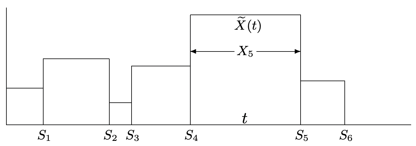
Let \(\widetilde{X}(t)\) be the duration of the inter-renewal interval containing time \(t\), i.e., \(\widetilde{X}(t)=X_{N(t)+1}=S_{N(t)+1}-S_{N(t)}\) (see Figure 4.8). It is clear that \(\widetilde{X}(t)=Z(t)+Y(t)\), and thus the time-average of the duration is given by

\[\lim _{t \rightarrow \infty} \frac{\int_{\tau=0}^{t} \widetilde{X}(\tau) d \tau}{t}=\frac{\mathrm{E}\left[X^{2}\right]}{\mathrm{E}[X]}\text{WP1}\label{4.17} \]

Again, long intervals are heavily weighted in this average, so that the time-average duration is at least as large as the mean inter-renewal interval and often much larger.

Figure 4.8: Duration \(\widetilde{X}(t)=X_{N(t)}\) of the inter-renewal interval containing \(t\).

General renewal-reward processes

In each of these examples, and in many other situations, we have a random function of time (i.e., \(Y(t)\), \(Z(t)\), or \(\tilde{X}(t)\)) whose value at time \(t\) depends only on where \(t\) is in the current inter-renewal interval (i.e., on the age \(Z(t)\) and the duration \(\widetilde{X}(t)\) of the current inter-renewal interval). We now investigate the general class of reward functions for which the reward at time \(t\) depends at most on the age and the duration at \(t\), i.e., the reward \(R(t)\) at time \(t\) is given explicitly as a function⁶ \(\mathcal{R}(Z(t), \widetilde{X}(t))\) of the age and duration at \(t\).

For the three examples above, the function \(\mathcal{R}\) is trivial. That is, the residual life, \(Y(t)\), is given by \(\widetilde{X}(t)-Z(t)\) and the age and duration are given directly.

We now find the time-average value of \(R(t)\), namely, \(\lim _{t \rightarrow \infty} \frac{1}{t} \int_{0}^{t} R(\tau) d \tau\). As in examples t 0 4.4.1 to 4.4.4 above, we first want to look at the accumulated reward over each inter-renewal period separately. Define \(\mathrm{R}_{n}\) as the accumulated reward in the nth renewal interval,

\[\mathrm{R}_{n}=\int_{S_{n-1}}^{S_{n}} R(\tau) d(\tau)=\int_{S_{n-1}}^{S_{n}} \mathcal{R}[Z(\tau), \widetilde{X}(\tau)] d \tau\label{4.18} \]

For residual life (see Example 4.4.1), \(\mathrm{R}_{n}\) is the area of the nth isosceles right triangle in Figure 4.5. In general, since \(Z(\tau)=\tau-S_{n-1}\),

\[\mathrm{R}_{n}=\int_{S_{n-1}}^{S_{n}} \mathcal{R}\left(\tau-S_{n-1}, X_{n}\right) d \tau=\int_{z=0}^{X_{n}} \mathcal{R}\left(z, X_{n}\right) d z\label{4.19} \]

Note that \(\mathrm{R}_{n}\) is a function only of \(X_{n}\), where the form of the function is determined by \(\mathcal{R}(Z, X)\). From this, it is clear that \(\left\{\mathrm{R}_{n} ; n \geq 1\right\}\) is essentially⁷ a set of IID random variables. For residual life, \(\mathcal{R}\left(z, X_{n}\right)=X_{n}-z\), so the integral in \ref{4.19} is \(X_{n}^{2} / 2\), as calculated by inspection before. In general, from (4.19), the expected value of \(\mathrm{R}_{n}\) is given by

\[\mathrm{E}\left[\mathrm{R}_{n}\right]=\int_{x=0}^{\infty} \int_{z=0}^{x} \mathcal{R}(z, x) d z\ d \mathrm{~F}_{X}(x)\label{4.20} \]

Breaking \(\int_{0}^{t} R(\tau) d \tau\) into the reward over the successive renewal periods, we get

\[\begin{aligned}
\int_{0}^{t} R(\tau) d \tau &=\int_{0}^{S_{1}} R(\tau) d \tau+\int_{S_{1}}^{S_{2}} R(\tau) d \tau+\cdots+\int_{S_{N(t)-1}}^{S_{N(t)}} R(\tau) d \tau+\int_{S_{N(t)}}^{t} R(\tau) d \tau \\
&=\sum_{n=1}^{N(t)} \mathrm{R}_{n}+\int_{S_{N(t)}}^{t} R(\tau) d \tau
\end{aligned}\label{4.21} \]

The following theorem now generalizes the results of Examples 4.4.1, 4.4.3, and 4.4.4 to general renewal-reward functions.

Theorem 4.4.1

Let \(\{R(t) ; t>0\} \geq 0\) be a nonnegative renewal-reward function for a renewal process with expected inter-renewal time \(\mathrm{E}[X]=\bar{X}<\infty\). If \(E\left[R_{n}\right]<\infty\), then with probability 1

\[\lim _{t \rightarrow \infty} \frac{1}{t} \int_{\tau=0}^{t} R(\tau) d \tau=\frac{\mathrm{E}\left[\mathrm{R}_{n}\right]}{\bar{X}}\label{4.22} \]

Proof

Using (4.21), the accumulated reward up to time \(t\) can be bounded between the accumulated reward up to the renewal before \(t\) and that to the next renewal after \(t\),

\[\frac{\sum_{n=1}^{N(t)} \mathrm{R}_{n}}{t} \leq \frac{\int_{\tau=0}^{t} R(\tau) d \tau}{t} \leq \frac{\sum_{n=1}^{N(t)+1} \mathrm{R}_{n}}{t}\label{4.23} \]

The left hand side of \ref{4.23} can now be broken into

\[\frac{\sum_{n=1}^{N(t)} \mathrm{R}_{n}}{t}=\frac{\sum_{n=1}^{N(t)} \mathrm{R}_{n}}{N(t)} \frac{N(t)}{t}\label{4.24} \]

Each \(\mathrm{R}_{n}\) is a given function of \(X_{n}\), so the \(\mathrm{R}_{n}\) are IID. As \(t \rightarrow \infty\), \(N(t) \rightarrow \infty\), and, thus, as we have seen before, the strong law of large numbers can be used on the first term on the right side of (4.24), getting \(\mathrm{E}\left[\mathrm{R}_{n}\right]\) with probability 1. Also the second term approaches \(1 / \bar{X}\) by the strong law for renewal processes. Since \(0<\bar{X}<\infty\) and \(\mathrm{E}\left[\mathrm{R}_{n}\right]\) is finite, the product of the two terms approaches the limit \(\mathrm{E}\left[\mathrm{R}_{n}\right] / \bar{X}\). The right-hand inequality of \ref{4.23} is handled in almost the same way,

\[\frac{\sum_{n=1}^{N(t)+1} \mathrm{R}_{n}}{t}=\frac{\sum_{n=1}^{N(t)+1} \mathrm{R}_{n}}{N(t)+1} \frac{N(t)+1}{N(t)} \frac{N(t)}{t}\label{4.25} \]

It is seen that the terms on the right side of \ref{4.25} approach limits as before and thus the term on the left approaches \[\mathrm{E}\left[\mathrm{R}_{n}\right] / \bar{X} \nonumber \] with probability 1. Since the upper and lower bound in \ref{4.23} approach the same limit, \((1 / t) \int_{0}^{t} R(\tau) d \tau\) approaches the same limit and the theorem is proved.

The restriction to nonnegative renewal-reward functions in Theorem 4.4.1 is slightly artificial. The same result holds for non-positive reward functions simply by changing the directions of the inequalities in (4.23). Assuming that \(\mathrm{E}\left[\mathrm{R}_{n}\right]\) exists (i.e., that both its positive and negative parts are finite), the same result applies in general by splitting an arbitrary reward function into a positive and negative part. This gives us the corollary:

Corollary 4.4.1

Let \(\{R(t) ; t>0\}\) be a renewal-reward function for a renewal process with expected inter-renewal time \(\mathrm{E}[X]=\bar{X}<\infty\). If \(\mathrm{E}\left[\mathrm{R}_{n}\right]\) exists, then with probability 1

\[\lim _{t \rightarrow \infty} \frac{1}{t} \int_{\tau=0}^{t} R(\tau) d \tau=\frac{\mathrm{E}\left[\mathrm{R}_{n}\right]}{\bar{X}}\label{4.26} \]

Example 4.4.5 (Distribution of Residual Life)

Example 4.4.1 treated the time-average value of the residual life \(Y(t)\). Suppose, however, that we would like to find the time-average distribution function of \(Y(t)\), i.e., the fraction of time that \(Y(t) \leq y\) as a function of \(y\). The approach, which applies to a wide variety of applications, is to use an indicator function (for a given value of \(y\)) as a reward function. That is, define \(R(t)\) to have the value 1 for all \(t\) such that \(Y(t) \leq y\) and to have the value 0 otherwise. Figure 4.9 illustrates this function for a given sample path. Expressing this reward function in terms of \(Z(t)\) and \(\widetilde{X}(t)\), we have

\(R(t)=\mathcal{R}(Z(t), \widetilde{X}(t))= \begin{cases}1 ; & \tilde{X}(t)-Z(t) \leq y \\ 0 ; & \text { otherwise }\end{cases}\)

Note that if an inter-renewal interval is smaller than \(y\) (such as the third interval in Figure 4.9), then \(R(t)\) has the value one over the entire interval, whereas if the interval is greater

Figure 4.9: Reward function to find the time-average fraction of time that \(\{Y(t) \leq y\}\). For the sample function in the figure, \(X_{1}>y, X_{2}>y\), and \(X_{4}>y\), but \(X_{3}<y\)

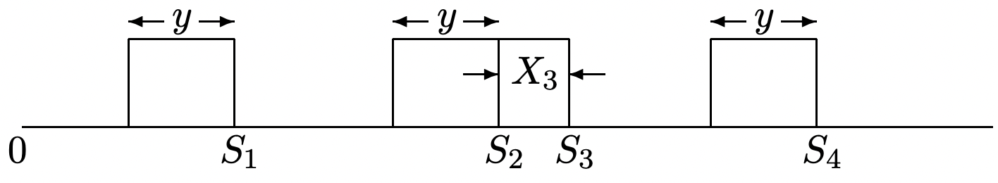
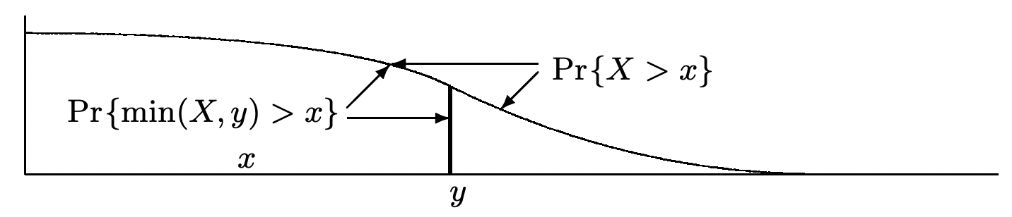
than \(y\), then \(R(t)\) has the value one only over the final \(y\) units of the interval. Thus \(\mathrm{R}_{n}=\min \left[y, X_{n}\right]\). Note that the random variable \(\min \left[y, X_{n}\right]\) is equal to \(X_{n}\) for \(X_{n} \leq y\), and thus has the same distribution function as \(X_{n}\) in the range 0 to \(y\). Figure 4.10 illustrates this in terms of the complementary distribution function. From the figure, we see that

\[\mathrm{E}\left[\mathrm{R}_{n}\right]=\mathrm{E}[\min (X, y)]=\int_{x=0}^{\infty} \operatorname{Pr}\{\min (X, y)>x\} d x=\int_{x=0}^{y} \operatorname{Pr}\{X>x\} d x\label{4.27} \]

Figure 4.10: \(\mathrm{R}_{n}\) for distribution of residual life.

Let \(\mathrm{F}_{Y}(y)=\lim _{t \rightarrow \infty}(1 / t) \int_{0}^{t} R(\tau) d \tau\) denote the time-average fraction of time that the residual life is less than or equal to \(y\). From Theorem 4.4.1 and Eq.(4.27), we then have

\[\mathrm{F}_{Y}(y)=\frac{\mathrm{E}\left[\mathrm{R}_{n}\right]}{\bar{X}}=\frac{1}{\bar{X}} \int_{x=0}^{y} \operatorname{Pr}\{X>x\} d x \quad \mathrm{WP} 1\label{4.28} \]

As a check, note that this integral is increasing in \(y\) and approaches 1 as \(y \rightarrow \infty\). Note also that the expected value of \(Y\), calculated from (4.28), is given by \(\mathrm{E}\left[X^{2}\right] / 2 \bar{X}\), in agreement with (4.15).

The same argument can be applied to the time-average distribution of age (see Exercise 4.12). The time-average fraction of time, \(\mathrm{F}_{Z}(z)\), that the age is at most \(z\) is given by

\[\mathrm{F}_{Z}(z)=\frac{1}{\bar{X}} \int_{x=0}^{z} \operatorname{Pr}\{X>x\} d x \quad{WP1}\label{4.29} \]

In the development so far, the reward function \(R(t)\) has been a function solely of the age and duration intervals, and the aggregate reward over the nth inter-renewal interval is a function only of \(X_{n}\). In more general situations, where the renewal process is embedded in some more complex process, it is often desirable to define \(R(t)\) to depend on other aspects of the process as well. The important thing here is for \(\left\{\mathrm{R}_{n} ; n \geq 1\right\}\) to be an IID sequence. How to achieve this, and how it is related to queueing systems, is described in Section 4.5.3. Theorem 4.4.1 clearly remains valid if \(\left\{\mathrm{R}_{n} ; n \geq 1\right\}\) is IID. This more general type of renewal-reward function will be required and further discussed in Sections 4.5.3 to Rss7 where we discuss Little’s theorem and the M/G/1 expected queueing delay, both of which use this more general structure.

Limiting time-averages are sometimes visualized by the following type of experiment. For some given large time \(t\), let \(T\) be a uniformly distributed random variable over \((0, t]\); \(T\) is independent of the renewal-reward process under consideration. Then \((1 / t) \int_{0}^{t} R(\tau) d \tau\) is the expected value (over \(T\)) of \(R(T)\) for a given sample path of \(\{R(\tau) ; \tau>0\}\). Theorem 4.4.1 states that in the limit \(t \rightarrow \infty\), all sample paths (except a set of probability 0) yield the same expected value over \(T\). This approach of viewing a time-average as a random choice of time is referred to as random incidence. Random incidence is awkward mathematically, since the random variable \(T\) changes with the overall time \(t\) and has no reasonable limit. It also blurs the distinction between time and ensemble-averages, so it will not be used in what follows.

---

⁵ \(\int_{0}^{t} Y(\tau) d \tau\) is a rv just like any other function of a set of rv’s. It has a sample value for each sample function of \(\{N(t) ; t>0\}\), and its distribution function could be calculated in a straightforward but tedious way. For arbitrary stochastic processes, integration and differentiation can require great mathematical sophistication, but none of those subtleties occur here.

⁶ This means that \(R(t)\) can be determined at any \(t\) from knowing \(Z(t)\) and \(X(t)\). It does not mean that \(R(t)\) must vary as either of those quantities are changed. Thus, for example, \(R(t)\) could depend on only one of the two or could even be a constant.

⁷ One can certainly define functions \(\mathcal{R}(Z, X)\) for which the integral in \ref{4.19} is infinite or undefined for some values of \(X_{n}\), and thus \(\mathrm{R}_{n}\) becomes a defective rv. It seems better to handle this type of situation when it arises rather than handling it in general.