4.3: Strong Law for Renewal Processes

To get an intuitive idea why \(N(t) / t\) should approach \(1 / \bar{X}\) for large \(t\), consider Figure 4.2. For any given sample function of \(\{N(t) ; t>0\}\), note that, for any given \(t\), \(N(t) / t \) is the slope of a straight line from the origin to the point \((t, N(t))\). As \(t\) increases, this slope decreases in the interval between each adjacent pair of arrival epochs and then jumps up at the next arrival epoch. In order to express this as an equation, note that \(t\) lies between the \(N(t)\) th arrival (which occurs at \(S_{N(t)}\)) and the \((N(t)+1)\)th arrival (which occurs at \(S_{N(t)+1}\)). Thus, for all sample points,

\[\frac{N(t)}{S_{N(t)}} \geq \frac{N(t)}{t}>\frac{N(t)}{S_{N(t)+1}}.\label{4.7} \]

Figure 4.2: Comparison of a sample function of \(N(t) / t\) with \(\frac{N(t)}{S_{N(t)}}\) and \(\frac{N(t)}{S_{N(t)+1}}\) for the same sample point. Note that for the given sample point, \(N(t)\) is the number of arrivals up to and including \(t\), and thus \(S_{N(t)}\) is the epoch of the last arrival before or at time \(t\). Similarly, \(S_{N(t)+1}\) is the epoch of the first arrival strictly after time \(t\).

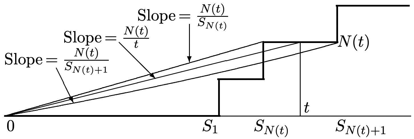
We want to show intuitively why the slope \(N(t) / t\) in the figure approaches \(1 / \bar{X}\) as \(t \rightarrow\infty\). As \(t\) increases, we would guess that \(N(t)\) increases without bound, i.e., that for each arrival, another arrival occurs eventually. Assuming this, the left side of \ref{4.7} increases with increasing \(t\) as \(1 / S_{1}, 2 / S_{2}, \ldots, n / S_{n}, \ldots\), where \(n=N(t)\). Since \(S_{n} / n\) converges to \(\bar{X}\) WP1 from the strong law of large numbers, we might be brave enough or insightful enough to guess that \(n / S_{n}\) converges to \(1 / \bar{X}\).

We are now ready to state the strong law for renewal processes as a theorem. Before proving the theorem, we formulate the above two guesses as lemmas and prove their validity.

Theorem 4.3.1 ( Strong Law for Renewal Processes).

For a renewal process with mean inter-renewal interval \(\bar{X}<\infty\), \(\lim _{t \rightarrow \infty} N(t) / t=1 / \bar{X}\) WP1.

Lemma 4.3.1

Let \(\{N(t) ; t>0\}\) be a renewal counting process with inter-renewal rv’s \(\left\{X_{n} ; n \geq 1\right\}\). Then (whether or not \(\bar{X}<\infty\)), \(\lim _{t \rightarrow \infty} N(t)=\infty\) WP1 and \(\lim _{t \rightarrow \infty} \mathrm{E}[N(t)]=\infty\).

Proof

Note that for each sample point \(\omega\), \(N(t, \omega)\) is a nondecreasing real-valued function of \(t\) and thus either has a finite limit or an infinite limit. Using (4.1), the probability that this limit is finite with value less than any given \(n\) is

\(\lim _{t \rightarrow \infty} \operatorname{Pr}\{N(t)<n\}=\lim _{t \rightarrow \infty} \operatorname{Pr}\left\{S_{n}>t\right\}=1-\lim _{t \rightarrow \infty} \operatorname{Pr}\left\{S_{n} \leq t\right\}\).

Since the \(X_{i}\) are rv’s, the sums \(S_{n}\) are also rv’s (i.e., nondefective) for each \(n\) (see Section 1.3.7), and thus \(\lim _{t \rightarrow \infty} \operatorname{Pr}\left\{S_{n} \leq t\right\}=1\) for each \(n\). Thus \(\lim _{t \rightarrow \infty} \operatorname{Pr}\{N(t)<n\}=0\) for each \(n\). This shows that the set of sample points \(\omega\) for which \(\lim _{t \rightarrow \infty} N(t(\omega))<n\) has probability 0 for all \(n\). Thus the set of sample points for which \(\lim _{t \rightarrow \infty} N(t, \omega)\) is finite has probability 0 and \(\lim _{t \rightarrow \infty} N(t)=\infty\) WP1.

Next, \(\mathrm{E}[N(t)]\) is nondecreasing in \(t\), and thus has either a finite or infinite limit as \(t \rightarrow \infty\). For each \(n\), \(\operatorname{Pr}\{N(t) \geq n\} \geq 1 / 2\) for large enough \(t\), and therefore \(\mathrm{E}[N(t)] \geq n / 2\) for such \(t\). Thus \(\mathrm{E}[N(t)]\) can have no finite limit as \(t \rightarrow \infty\), and \(\lim _{t \rightarrow \infty} \mathrm{E}[N(t)]=\infty\).

The following lemma is quite a bit more general than the second guess above, but it will be useful elsewhere. This is the formalization of the technique used at the end of the proof of the SLLN.

Lemma 4.3.2

Let \(\left\{Z_{n} ; n \geq 1\right\}\) be a sequence of rv’s such that \(\lim _{n \rightarrow \infty} Z_{n}=\alpha\) WP1. Let \(f\) be a real valued function of a real variable that is continuous at \(\alpha\). Then

\[\lim _{n \rightarrow \infty} f\left(Z_{n}\right)=f(\alpha) \quad \text{WP1}.\label{4.8} \]

Proof

First let \(z_{1}, z_{2}, \ldots\), be a sequence of real numbers such that \(\lim _{n \rightarrow \infty} z_{n}=\alpha\). Continuity of \(f\) at \(\alpha\) mean that for every \(\epsilon>0\), there is a \(\delta>0\) such that \(|f(z)-f(\alpha)|<\epsilon\) for all \(z\) such that \(|z-\alpha|<\delta\). Also, since \(\lim _{n \rightarrow \infty} z_{n}=\alpha\), we know that for every \(\delta>0\), there is an \(m\) such that \(\left|z_{n}-\alpha\right| \leq \delta\) for all \(n \geq m\). Putting these two statements together, we know that for every \(\epsilon>0\), there is an m such that \(\left|f\left(z_{n}\right)-f(\alpha)\right|<\epsilon\) for all \(n \geq m\). Thus \(\lim _{n \rightarrow \infty} f\left(z_{n}\right)=f(\alpha)\).

If \(\omega\) is any sample point such that \(\lim _{n \rightarrow \infty} Z_{n}(\omega)=\alpha\), then \(\lim _{n \rightarrow \infty} f\left(Z_{n}(\omega)\right)=f(\alpha)\). Since this set of sample points has probability 1, \ref{4.8} follows.

Proof of Theorem 4.3.1, Strong law for renewal processes:

Since \(\operatorname{Pr}\{X>0\}=1\) for a renewal process, we see that \(\bar{X}>0\). Choosing \(f(x)=1 / x\), we see that \(f(x)\) is continuous at \(x=\bar{X}\). It follows from Lemma 4.3.2 that

\(\lim _{n \rightarrow \infty} \frac{n}{S_{n}}=\frac{1}{\bar{X}} \quad \text{WP1}.\)

From Lemma 4.3.1, we know that \(\lim _{t \rightarrow \infty} N(t)=\infty\) with probability 1, so, with probability 1, \(N(t)\) increases through all the nonnegative integers as \(t\) increases from 0 to \(\infty\). Thus

\(\lim _{t \rightarrow \infty} \frac{N(t)}{S_{N(t)}}=\lim _{n \rightarrow \infty} \frac{n}{S_{n}}=\frac{1}{\bar{X}}\quad \text{WP1}.\)

Recall that \(N(t) / t\) is sandwiched between \(N(t) / S_{N(t)}\) and \(N(t) / S_{N(t)+1}\), so we can complete the proof by showing that \(\lim _{t \rightarrow \infty} N(t) / S_{N(t)+1}=1 / \bar{X}\). To show this,

\(\lim _{t \rightarrow \infty} \frac{N(t)}{S_{N(t)+1}}=\lim _{n \rightarrow \infty} \frac{n}{S_{n+1}}=\lim _{n \rightarrow \infty} \frac{n+1}{S_{n+1}} \frac{n}{n+1}=\frac{1}{\bar{X}} \quad \text{WP1}.\)

We have gone through the proof of this theorem in great detail, since a number of the techniques are probably unfamiliar to many readers. If one reads the proof again, after becoming familiar with the details, the simplicity of the result will be quite striking. The theorem is also true if the mean inter-renewal interval is infinite; this can be seen by a truncation argument (see Exercise 4.8).

As explained in Section 4.2.1, Theorem 4.3.1 also implies the corresponding weak law of large numbers for \(N(t)\), i.e., for any \(\epsilon>0\), \(\lim _{t \rightarrow \infty} \operatorname{Pr}\{|N(t) / t-1 / \bar{X}| \geq \epsilon\}=0\)). This weak law could also be derived from the weak law of large numbers for \(S_{n}\) (Theorem 1.5.3). We do not pursue that here, since the derivation is tedious and uninstructive. As we will see, it is the strong law that is most useful for renewal processes.

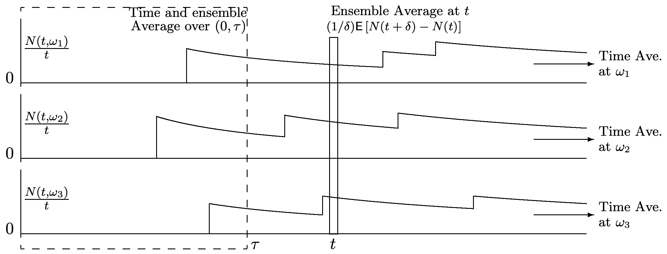
Figure 4.3 helps give some appreciation of what the strong law for \(N(t)\) says and doesn’t say. The strong law deals with time-averages, \(\lim _{t \rightarrow \infty} N(t, \omega) / t\), for individual sample points \(\omega\); these are indicated in the figure as horizontal averages, one for each \(\omega\). It is also of interest to look at time and ensemble-averages, \(\mathrm{E}[N(t) / t]\), shown in the figure as vertical averages. Note that \(N(t, \omega) / t\) is the time-average number of renewals from 0 to \(t\), whereas \(\mathrm{E}[N(t) / t]\) averages also over the ensemble. Finally, to focus on arrivals in the vicinity of a particular time \(t\), it is of interest to look at the ensemble-average \(E[N(t+\delta)-N(t)] / \delta\).

Given the strong law for \(N(t)\), one would hypothesize that \(\mathrm{E}[N(t) / t]\) approaches \(1 / \bar{X}\) as \(t \rightarrow \infty\). One might also hypothesize that \(\lim _{t \rightarrow \infty} \mathrm{E}[N(t+\delta)-N(t)] / \delta=1 / \bar{X}\), subject to some minor restrictions on \(\delta\). These hypotheses are correct and are discussed in detail in what follows. This equality of time-averages and limiting ensemble-averages for renewal processes carries over to a large number of stochastic processes, and forms the basis of ergodic theory. These results are important for both theoretical and practical purposes. It is sometimes easy to find time averages (just like it was easy to find the time-average \(N(t, \omega) / t\) from the strong law of large numbers), and it is sometimes easy to find limiting ensemble-averages. Being able to equate the two then allows us to alternate at will between time and ensemble-averages.

Figure 4.3: The time average at a sample point \(\omega\), the time and ensemble average from 0 to a given \(\tau\), and the ensemble-average in an interval \((t, t+\delta]\).

Note that in order to equate time-averages and limiting ensemble-averages, quite a few conditions are required. First, the time-average must exist in the limit \(t \rightarrow \infty\) with probability one and also have a fixed value with probability one; second, the ensemble-average must approach a limit as \(t \rightarrow \infty\); and third, the limits must be the same. The following example, for a stochastic process very different from a renewal process, shows that equality between time and ensemble averages is not always satisfied for arbitrary processes.

Example 4.3.1

Let \(\left\{X_{i} ; i \geq 1\right\}\) be a sequence of binary IID random variables, each taking the value 0 with probability 1/2 and 2 with probability 1/2. Let \(\left\{M_{n} ; n \geq 1\right\}\) be the product process in which \(M_{n}=X_{1} X_{2} \cdots X_{n}\). Since \(M_{n}=2^{n}\) if \(X_{1}\) to \(X_{n}\) each take the value 2 (an event of probability \(2^{-n}\)) and \(M_{n}=0\) otherwise, we see that \(\lim _{n \rightarrow \infty} M_{n}=0\) with probability 1. Also \(\mathrm{E}\left[M_{n}\right]=1\) for all \(n \geq 1\). Thus the time-average exists and equals 0 with probability 1 and the ensemble-average exists and equals 1 for all \(n\), but the two are different. The problem is that as \(n\) increases, the atypical event in which \(M_{n}=2^{n}\) has a probability approaching 0, but still has a significant effect on the ensemble-average.

Further discussion of ensemble averages is postponed to Section 4.6. Before that, we briefly state and discuss the central limit theorem for counting renewal processes and then introduce the notion of rewards associated with renewal processes.

Theorem 4.3.2 (Central Limit Theorem (CLT) for \(N(t)\)).

Assume that the interrenewal intervals for a renewal counting process \(\{N(t) ; t>0\}\) have finite standard deviation \(\sigma>0\). Then

\[\lim _{t \rightarrow \infty} \operatorname{Pr}\left\{\frac{N(t)-t / \bar{X}}{\sigma \bar{X}^{-3 / 2} \sqrt{t}}<\alpha\right\}=\Phi(\alpha).\label{4.9} \]

where \(\Phi(y)=\int_{-\infty}^{y} \frac{1}{\sqrt{2 \pi}} \exp \left(-x^{2} / 2\right) d x\).

This says that the distribution function of \(N(t)\) tends to the Gaussian distribution with mean \(t / \bar{X}\) and standard deviation \(\sigma \bar{X}^{-3 / 2} \sqrt{t}\).

Figure 4.4: Illustration of the central limit theorem (CLT) for renewal processes. A given integer \(n\) is shown on the vertical axis, and the corresponding mean, \(\mathrm{E}\left[S_{n}\right]=n \bar{X}\) is shown on the horizontal axis. The horizontal line with arrows at height \(n\) indicates \(\alpha\) standard deviations from \(\mathrm{E}\left[S_{n}\right]\), and the vertical line with arrows indicates the distance below \((t / \bar{X})\).

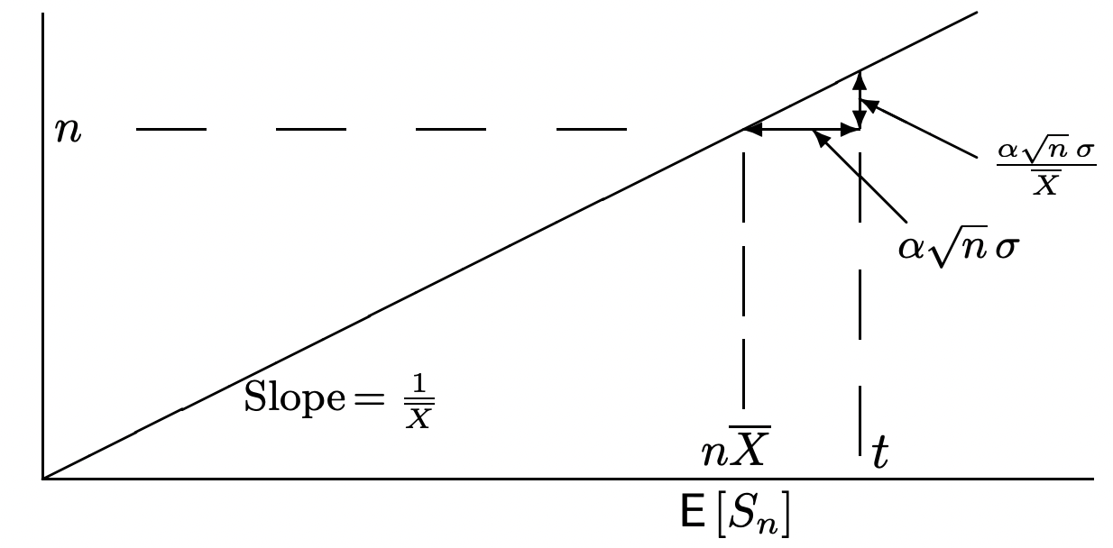
The theorem can be proved by applying Theorem 1.5.2 (the CLT for a sum of IID rv’s) to \(S_{n}\) and then using the identity \(\left\{S_{n} \leq t\right\}=\{N(t) \geq n\}\). The general idea is illustrated in Figure 4.4, but the details are somewhat tedious, and can be found, for example, in [16]. We simply outline the argument here. For any real \(\alpha\), the CLT states that

\(\operatorname{Pr}\left\{S_{n} \leq n \bar{X}+\alpha \sqrt{n} \sigma\right\} \approx \Phi(\alpha)\),

where