4.7: Renewal-reward Processes and Ensemble-averages

Theorem 4.4.1 showed that if a renewal-reward process has an expected inter-renewal interval \(\overline{X}\) and an expected inter-renewal reward \(\mathrm{E}\left[R_{n}\right]\), then the time-average reward is \(\mathrm{E}\left[R_{n}\right] / \overline{X}\) with probability 1. In this section, we explore the ensemble average, \(\mathrm{E}[R(t)]\), as a function of time \(t\). It is easy to see that \(\mathrm{E}[R(t)]\) typically changes with \(t\), especially for small \(t\), but a question of major interest here is whether \(\mathrm{E}[R(t)]\) approaches a constant as \(t \rightarrow \infty\).

In more concrete terms, if the arrival times of busses at a bus station forms a renewal process, then the waiting time for the next bus, i.e., the residual life, starting at time \(t\), can be represented as a reward function \(R(t)\). We would like to know if the expected waiting time depends critically on \(t\), where \(t\) is the time since the renewal process started, i.e., the time since a hypothetical bus number 0 arrived. If \(\mathrm{E}[R(t)]\) varies significantly with \(t\), even as \(t \rightarrow \infty\), it means that the choice of \(t=0\) as the beginning of the initial interarrival interval never dies out as \(t \rightarrow \infty\).

Blackwell’s renewal theorem (and common sense) tell us that there is a large difference between arithmetic inter-renewal times and non-arithmetic inter-renewal times. For the arithmetic case, all renewals occur at multiples of the span \(\lambda\). Thus, for example, the expected waiting time (i.e., the expected residual life) decreases at rate 1 from each multiple of \(\lambda\) to the next, and it increases with a jump equal to the probability of an arrival at each multiple of \(\lambda\). For this reason, we usually consider various reward functions only at multiples of \(\lambda\). We would guess, then, that \(\mathrm{E}[R(n \lambda)]\) approaches a constant as \(n \rightarrow \infty\).

For the non-arithmetic case, on the other hand, the expected number of renewals in any small interval of length \(\delta\) becomes independent of \(t\) as \(t \rightarrow \infty\), so we might guess that \(\mathrm{E}[R(t)]\) approaches a limit as \(t \rightarrow \infty\). We would also guess that these asymptotic ensemble averages are equal to the appropriate time averages from Section 4.4.

The bottom line for this section is that under very broad conditions, the above guesses are essentially correct. Thus the limit as \(t \rightarrow \infty\) of a given ensemble-average reward can usually be computed simply by finding the time-average and vice-versa. Sometimes time-averages are simpler, and sometimes ensemble-averages are. The advantage of the ensemble-average approach is both the ability to find \(\mathrm{E}[R(t)]\) for finite values of \(t\) and to understand the rate of convergence to the asymptotic result.

The following subsection is restricted to the arithmetic case. We will derive the joint distribution function of age and duration for any given time \(t\), and then look at the limit as \(t \rightarrow \infty\). This leads us to arbitrary reward functions (such as residual life) for the arithmetic case. We will not look specifically at generalized reward functions that depend on other processes, but this generalization is quite similar to that for time-averages.

The non-arithmetic case is analyzed in the remainder of the subsections of this section. The basic ideas are the same as the arithmetic case, but a number of subtle mathematical limiting issues arise. The reader is advised to understand the arithmetic case first, since the limiting issues in the non-arithmetic case can then be viewed within the intuitive context of the arithmetic case.

duration for arithmetic processes

Let \(\{N(t) ; t>0\}\) be an arithmetic renewal counting process with inter-renewal intervals \(X_{1}, X_{2}, \ldots\) and arrival epochs \(S_{1}, S_{2}, \ldots\), where \(S_{n}=X_{1}+\cdots+X_{n}\). To keep the notation as uncluttered as possible, we take the span to be one and then scale to an arbitrary \(\lambda\) later. Thus each \(X_{i}\) is a positive integer-valued rv.

Recall that the age \(Z(t)\) at any given \(t>0\) is \(Z(t)=t-S_{N(t)}\) (where by convention \(S_{0}=0\)) and the duration \(\widetilde{X}(t)\) is \(\widetilde{X}(t)=S_{N(t)+1}(t)-S_{N(t)}\). Since arrivals occur only at integer times, we initially consider age and duration only at integer times also. If an arrival occurs at integer time \(t\), then \(S_{N(t)}=t\) and \(Z(t)=0\). Also, if \(S_{1}>t\), then \(N(t)=0\) and \(Z(t)=t\) (i.e., the age is taken to be \(t\) if no arrivals occur up to and including time \(t\)). Thus, for integer \(t\), \(Z(t)\) is an integer-valued rv taking values from \([0, t]\). Since \(S_{N(t)+1}>t\), it follows that \(\widetilde{X}(t)\) is an integer-valued rv satisfying \(\widetilde{X}(t)>Z(t)\). Since both are integer valued, \(\widetilde{X}(t)\) must exceed \(Z(t)\) by at least 1 (or by \(\lambda\) in the more general case of span \(\lambda\)).

In order to satisfy \(Z(t)=i\) and \(\tilde{X}(t)=k\) for given \(i<t\), it is necessary and sufficient to have an arrival epoch at \(t-i\) followed by an interarrival interval of length \(k\), where \(k \geq i+1\). For \(Z(t)=t\) and \(\widetilde{X}(t)=k\), it is necessary and sufficient that \(k>t\), i.e., that the first inter-renewal epoch occurs at \(k>t\).

Theorem 4.7.1

Let \(\left\{X_{n} ; n \geq 1\right\}\) be the interarrival intervals of an arithmetic renewal process with unit span. Then the the joint PMF of the age and duration at integer time \(t \geq 1\) is given by

\[\mathbf{p}_{Z(t), \tilde{X}(t)}(i, k)= \begin{cases}\mathbf{p}_{X}(k) & \text { for } i=t, k>t \\ q_{t-i} \mathbf{p}_{X}(k) & \text { for } 0 \leq i<t, k>i. \\ 0 & \text { otherwise }\end{cases}\label{4.62} \]

where \(q_{j}=\operatorname{Pr}\{\text { arrival at time } j\}\). The limit as \(t \rightarrow \infty\) for any given \(0 \leq i<k\) is given by

\[\lim _{\text {integer } t \rightarrow \infty} \mathrm{p}_{Z(t), \widetilde{X}(t)}(i, k)=\frac{\mathrm{p}_{X}(k)}{\overline{X}}.\label{4.63} \]

Proof

The idea is quite simple. For the upper part of (4.62), note that the age is \(t\) if and only there are no arrivals in \((0, t]\), which corresponds to \(X_{1}=k\) for some \(k>t\). For the middle part, the age is \(i\) for a given \(i<t\) if and only if there is an arrival at \(t-i\) and the next arrival epoch is after \(t\), which means that the corresponding interarrival interval \(k\) exceeds \(i\). The probability of an arrival at \(t-i\), i.e., \(q_{t-i}\), depends only on the arrival epochs up to and including time \(t-i\), which should be independent of the subsequent interarrival time, leading to the product in the middle term of (4.62). To be more precise about this independence, note that for \(i<t\),

\[q_{t-i}=\operatorname{Pr}\{\operatorname{arrival} \operatorname{at} t-i\}=\sum_{n \geq 1} \mathrm{p}_{S_{n}}(t-i)\label{4.64} \]

Given that \(S_{n}=t-i\), the probability that \(X_{n+1}=k\) is \(\mathrm{p}_{X}(k)\). This is the same for all \(n\), establishing (4.62).

For any fixed \(i\), \(k\) with \(i<k\), note that only the middle term in \ref{4.62} is relevant as \(t \rightarrow \infty\). Using Blackwell’s theorem \ref{4.61} to take the limit as \(t \rightarrow \infty\), we get (4.63)

The probabilities in the theorem, both for finite \(t\) and asymptotically as \(t \rightarrow \infty\), are illustrated in Figure 4.17. The product form of the probabilities in \ref{4.62} (as illustrated in the figure) might lead one to think that \(Z(t)\) and \(\widetilde{X}(t)\) are independent, but this is incorrect because of the constraint that \(\widetilde{X}(t)>Z(t)\). It is curious that in the asymptotic case, \ref{4.63} shows that, for a given duration \(\tilde{X}(t)=k\), the age is equally likely to have any integer value from 0 to \(k-1\), i.e., for a given duration, the interarrival interval containing \(t\) is uniformly distributed around \(t\).

The marginal PMF for \(Z(t)\) is calculated below using (4.62).

\[\mathrm{p}_{Z(t)}(i)= \begin{cases}\mathrm{F}_{X}^{\mathrm{c}}(i) & \text { for } i=t \\ q_{t-i} \mathrm{~F}_{X}^{\mathrm{c}}(i) & \text { for } 0 \leq i<t. \\ 0 & \text { otherwise }\end{cases}\label{4.65} \]

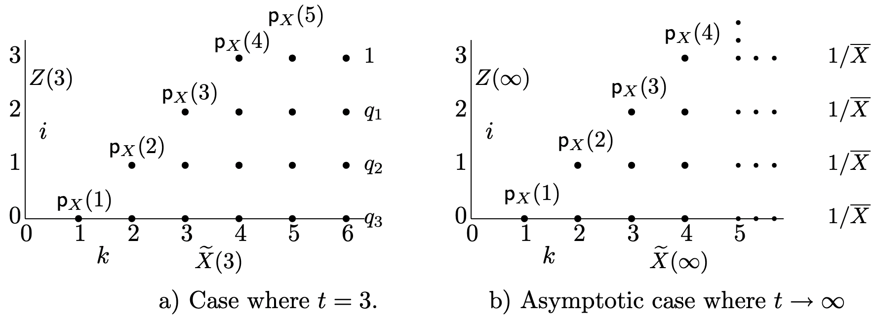
Figure 4.17: Joint PMF, \(\mathrm{p}_{\tilde{X}(t) Z(t)}(k, i)\) of \(\widetilde{X}(t)\) and \(Z(t)\) in an arithmetic renewal in an arithmetic renewal process with span 1. In part a), \(t=3\) and the PMF at each sample point is the product of two terms, \(q_{t-i}=\operatorname{Pr}\{\text { Arrival at } t-i\}\) and \(\mathrm{p}_{X}(k)\). Part b) is the asymptotic case where \(t \rightarrow \infty\). Here the arrival probabilities become uniform.

where \(\mathrm{F}_{X}^{c}(i)=\mathrm{p}_{X}(i+1)+\mathrm{p}_{X}(i+2)+\cdots\). The marginal PMF for \(\widetilde{X}(t)\) can be calculated directly from (4.62), but it is simplified somewhat by recognizing that

\[q_{j}=m(j)-m(j-1).\label{4.66} \]

Substituting this into \ref{4.62} and summing over age,

\[\mathrm{p}_{\tilde{X}(t)}(k)= \begin{cases}\mathrm{p}_{X}(k)[m(t)-m(t-k)] & \text { for } k<t \\ \mathrm{p}_{X}(k) m(t) & \text { for } k=t. \\ \mathrm{p}_{X}(k)[m(t)+1] & \text { for } k>t\end{cases}\label{4.67} \]

The term +1 in the expression for \(k>t\) corresponds to the uppermost point for the given \(k\) in Figure 4.17a. This accounts for the possibility of no arrivals up to time \(t\). It is not immediately evident that \(\sum_{k} \mathrm{p}_{\tilde{X}(t)}(k)=1\), but this can be verified from the renewal equation, (4.52).

Blackwell’s theorem shows that the arrival probabilities tend to \(1 / \overline{X}\) as \(t \rightarrow \infty\), so the limiting marginal probabilities for age and duration become

\[\lim _{\text {integer } t \rightarrow \infty} \mathrm{p}_{Z(t)}(i)=\frac{\mathrm{F}_{X}^{\mathrm{c}}(i)}{\overline{X}}.\label{4.68} \]

\[\lim _{\text {integer } t \rightarrow \infty} \mathrm{p}_{\widetilde{X}(t)}(k)=\frac{k\ \mathrm{p}_{X}(k)}{\overline{X}}.\label{4.69} \]

The expected value of \(Z(t)\) and \(\widetilde{X}(t)\) can also be found for all \(t\) from \ref{4.62} and \ref{4.63} respectively, but they don’t have a particularly interesting form. The asymptotic values as \(t \rightarrow \infty\) are more simple and interesting. The asymptotic expected value for age is derived below from (4.68).²²

\[\begin{aligned}
\lim _{\text {integer } t \rightarrow \infty} \mathrm{E}[Z(t)] &=\sum_{i} i \lim _{\text {integer } t \rightarrow \infty} \mathrm{p}_{Z(t)}(i) \\
&=\frac{1}{\overline{X}} \sum_{i=1}^{\infty} \sum_{j=i+1}^{\infty} i \mathrm{p}_{X}(j)=\frac{1}{\overline{X}} \sum_{j=2}^{\infty} \sum_{i=1}^{j-1} i \mathrm{p}_{X}(j) \\
&=\frac{1}{\overline{X}} \sum_{j=2}^{\infty} \frac{j(j-1)}{2} \mathrm{p}_{X}(j) \\
&=\frac{\mathrm{E}\left[X^{2}\right]}{2 \overline{X}}-\frac{1}{2}.
\end{aligned}\label{4.70} \]

This limiting ensemble average age has the same dependence on \(\mathrm{E}\left[X^{2}\right]\) as the time average in (4.16), but, perhaps surprisingly, it is reduced from that amount by 1/2. To understand this, note that we have only calculated the expected age at integer values of \(t\). Since arrivals occur only at integer values, the age for each sample function must increase with unit slope as \(t\) is increased from one integer to the next. The expected age thus also increases, and then at the next integer value, it drops discontinuously due to the probability of an arrival at that next integer. Thus the limiting value of \(\mathrm{E}[Z(t)]\) has a saw tooth shape and the value at each discontinuity is the lower side of that discontinuity. Averaging this asymptotic expected age over a unit of time, the average is \(\mathrm{E}\left[X^{2}\right] / 2 \overline{X}\), in agreement with (4.16).

As with the time average, the limiting expected age is infinite if \(\mathrm{E}\left[X^{2}\right]=\infty\). However, for each \(t\), \(Z(t) \leq t\), so \(\mathrm{E}[Z(t)]<\infty\) for all \(t\), increasing without bound as \(t \rightarrow \infty\)

The asymptotic expected duration is derived in a similar way, starting from (4.69)

\[\begin{aligned}
\lim _{\text {integer } t \rightarrow \infty} \mathrm{E}[\tilde{X}(t)] &=\sum_{k} \lim _{\text {integer } t \rightarrow \infty} k \mathrm{p}_{\tilde{X}(t)}(k) \\
&=\sum_{k} \frac{k^{2} \mathrm{p}_{X}(k)}{\overline{X}}=\frac{\mathrm{E}\left[X^{2}\right]}{\overline{X}}.
\end{aligned}\label{4.71} \]

This agrees with the time average in (4.17). The reduction by 1/2 seen in \ref{4.70} is not present here, since as \(t\) is increased in the interval \([t, t+1), X(t)\) remains constant.

Since the asymptotic ensemble-average age differs from the time-average age in only a trivial way, and the asymptotic ensemble-average duration is the same as the time-average duration, it might appear that we have gained little by this exploration of ensemble averages. What we have gained, however, is a set of results that apply to all \(t\). Thus they show how (in principle) these results converge as \(t \rightarrow \infty\).

Joint age and duration: non-arithmetic case

Non-arithmetic renewal processes are mathematically more complicated than arithmetic renewal processes, but the concepts are the same. We start by looking at the joint probability of the age and duration, each over an incremental interval. (see Figure 4.18 (a)).

Figure 4.18: Part (a): The incremental square region \(A\) of sample values for \(Z(t)\) and \(\widetilde{X}(t)\) whose joint probability is specified in (4.73). The square is assumed to be inside the indicated semi-infinite trapezoidal region, i.e., to satisfy \(0 \leq z<z+\delta \leq t\) and \(z+2 \delta \leq x\). Part (b): Summing over discrete sample regions of \(\widetilde{X}(t)\) to find the marginal probability \(\operatorname{Pr}\{z \leq Z(t)<z+\delta\}=\operatorname{Pr}\{T\}+\operatorname{Pr}\{B\}\), where \(T\) is the triangular area and \(B\) the set of indicated squares.

Theorem 4.7.2

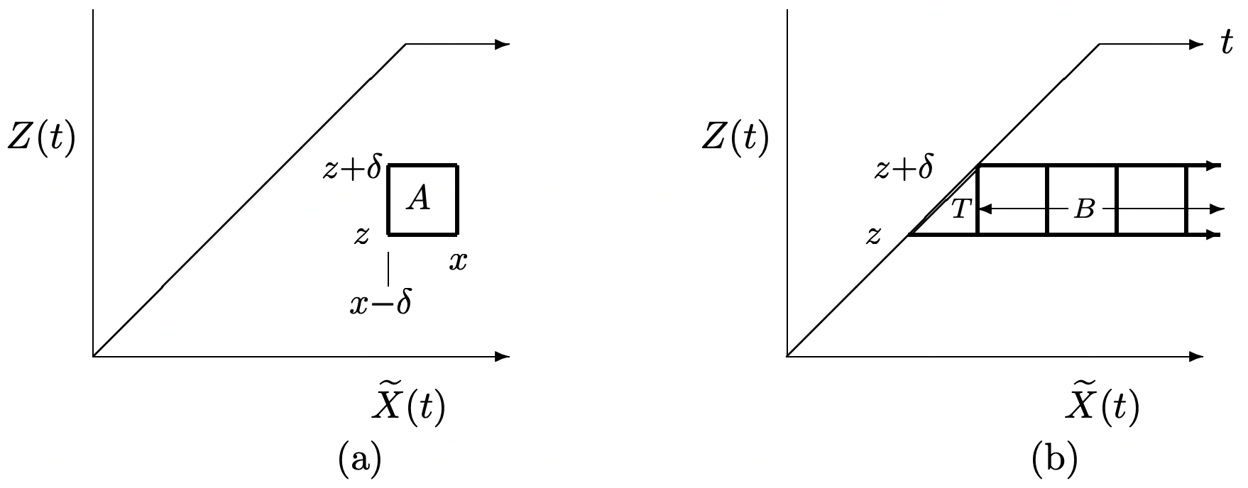
Consider an arbitrary renewal process with age \(Z(t)\) and duration \(\widetilde{X}(t)\) at any given time \(t>0\). Let \(A\) be the event

\[A=\{z \leq Z(t)<z+\delta\} \bigcap\{x-\delta<\widetilde{X}(t) \leq x\}, \label{4.72} \]

where \(0 \leq z<z+\delta \leq t\) and \(z+2 \delta \leq x\). Then

\[\operatorname{Pr}\{A\}=[m(t-z)-m(t-z-\delta)]\left[\mathrm{F}_{X}(x)-\mathrm{F}_{X}(x-\delta)\right]\label{4.73} \]

If in addition the renewal process is non-arithmetic,

\[\lim _{t \rightarrow \infty} \operatorname{Pr}\{A\}=\frac{\left[\mathrm{F}_{X}(x)-\mathrm{F}_{X}(x-\delta)\right]}{\overline{X}}\label{4.74} \]

Proof

Note that \(A\) is the box illustrated in Figure 4.18 \ref{a} and that under the given conditions, \(\tilde{X}(t)>Z(t)\) for all sample points in \(A\). Recall that \(Z(t)=t-S_{N(t)}\) and \(\tilde{X}(t)=S_{N(t)+1}-S_{N(t)}=X_{N(t)+1}\), so \(A\) can also be expressed as

\[A=\left\{t-z-\delta<S_{N(t)} \leq t-z\right\} \bigcap\left\{x-\delta<X_{N(t)+1} \leq x\right\}.\label{4.75} \]

We now argue that \(A\) can also be rewritten as

\[A=\bigcup_{n=1}^{\infty}\left\{\left\{t-z-\delta<S_{n} \leq t-z\right\} \bigcap\left\{x-\delta<X_{n+1} \leq x\right\}\right\}.\label{4.76} \]

To see this, first assume that the event in \ref{4.75} occurs. Then \(N(t)\) must have some positive sample value \(n\), so \ref{4.76} occurs. Next assume that the event in \ref{4.76} occurs, which means that one of the events, say the \(n\)th, in the union occurs. Since \(S_{n+1}=S_{n}+X_{n+1}>t\), we see that \(n\) is the sample value of \(S_{N(t)}\) and \ref{4.75} must occur.

To complete the proof, we must find \(\operatorname{Pr}\{A\}\). First note that \(A\) is a union of disjoint events. That is, although more than one arrival epoch might occur in \((t-z-\delta, t-z]\), the following arrival epoch can exceed \(t\) for only one of them. Thus

\[\operatorname{Pr}\{A\}=\sum_{n=1}^{\infty} \operatorname{Pr}\left\{\left\{t-z-\delta<S_{n} \leq t-z\right\} \bigcap\left\{x-\delta<X_{n+1} \leq x\right\}\right\}.\label{4.77} \]

For each \(n\), \(X_{n+1}\) is independent of \(S_{n}\), so

\(\begin{aligned}
\operatorname{Pr}\{\{t-z-\delta<&\left.\left.S_{n} \leq t-z\right\} \bigcap\left\{x-\delta<X_{n+1} \leq x\right\}\right\} \\
&=\operatorname{Pr}\left\{t-z-\delta<S_{n} \leq t-z\right\}\left[\mathrm{F}_{X}^{c}(x)-\mathrm{F}_{X}^{c}(x-\delta]\right..
\end{aligned}\)

Substituting this into \ref{4.77} and using \ref{4.51} to sum the series, we get

\(\operatorname{Pr}\{A\}=[m(t-z)-m(t-z-\delta)]\left[\mathrm{F}_{X}(x)-\mathrm{F}_{X}(x-\delta)\right]\).

This establishes (4.73). Blackwell’s theorem then establishes (4.74).

It is curious that \(\operatorname{Pr}\{A\}\) has such a simple product expression, where one term depends only on the function \(m(t)\) and the other only on the distribution function \(\mathrm{F}_{X}\). Although the theorem is most useful as \(\delta \rightarrow 0\), the expression is exact for all δ such that the square region \(A\) satisfies the given constraints (i.e., \(A\) lies in the indicated semi-infinite trapezoidal region).

Z(t) for finite t: non-arithmetic case

In this section, we first use Theorem 4.7.2 to find bounds on the marginal incremental probability of \(Z(t)\). We then find the distribution function, \(\mathrm{F}_{Z(t)}(z)\), and the expected value, \(\mathrm{E}[Z(t)]\) of \(Z(t)\).

Corollary 4.7.1.

For \(0 \leq z<z+\delta \leq t\), the following bounds hold on \(\operatorname{Pr}\{z \leq Z(t)<z+\delta\}\).

\[\operatorname{Pr}\{z \leq Z(t)<z+\delta\} \geq[m(t-z)-m(t-z-\delta)] \mathrm{F}_{X}^{c}(z+\delta)\label{4.78} \]

\[\operatorname{Pr}\{z \leq Z(t)<z+\delta\} \leq[m(t-z)-m(t-z-\delta)] \mathrm{F}_{X}^{\mathrm{c}}(z).\label{4.79} \]

Proof

As indicated in Figure 4.18 (b), \(\operatorname{Pr}\{z \leq Z(t)<z+\delta\}=\operatorname{Pr}\{T\}+\operatorname{Pr}\{B\}\), where \(T\) is the triangular region,

\(T=\{z \leq Z(t)<z+\delta\} \bigcap\{Z(t)<\tilde{X}(t) \leq z+\delta\}\),

and \(B\) is the rectangular region

\(B=\{z \leq Z(t)<z+\delta\} \bigcap\{\widetilde{X}(t)>z+\delta\}\).

It is easy to find \(\operatorname{Pr}\{B\}\) by summing the probabilities in \ref{4.73} for the squares indicated in Figure 4.18 (b). The result is

\[\operatorname{Pr}\{B\}=[m(t-z)-m(t-z-\delta)] \mathrm{F}_{X}^{\mathrm{c}}(z+\delta)\label{4.80} \]

Since \(\operatorname{Pr}\{T\} \geq 0\), this establishes the lower bound in (4.78). We next need an upper bound to \(\operatorname{Pr}\{T\}\) and start by finding an event that includes \(T\).

\(\begin{aligned}
T &=\{z \leq Z(t)<z+\delta\} \bigcap\{Z(t)<\widetilde{X}(t) \leq z+\delta\} \\
&=\bigcup_{n \geq 1}\left[\left\{t-z-\delta<S_{n} \leq t-z\right\} \bigcap\left\{t-S_{n}<X_{n+1} \leq z+\delta\right\}\right] \\
& \subseteq \bigcup_{n \geq 1}\left[\left\{t-z-\delta<S_{n} \leq t-z\right\} \bigcap\left\{z<X_{n+1} \leq z+\delta\right\}\right],
\end{aligned}\)

where the inclusion follows from the fact that \(S_{n} \leq t-z\) for the event on the left to occur, and this implies that \(z \leq t-S_{n}\).

Using the union bound, we then have

\(\begin{aligned}
\operatorname{Pr}\{T\} & \leq\left[\sum_{n \geq 1} \operatorname{Pr}\left\{\left\{t-z-\delta<S_{n} \leq t-z\right\}\right]\left[\mathrm{F}_{X}^{c}(z)-\mathrm{F}_{X}^{c}(z+\delta)\right]\right.\\
&=[m(t-z)-m(t-z-\delta)]\left[\mathrm{F}_{X}^{c}(z)-\mathrm{F}_{X}^{c}(z+\delta)\right] .
\end{aligned}\)

Combining this with (4.80), we have (4.79).

The following corollary uses Corollary 4.7.1 to determine the distribution function of \(Z(t)\). The rather strange dependence on the existence of a Stieltjes integral will be explained after the proof.

Corollary 4.7.2

If the Stieltjes integral \(\int_{t-z}^{t} \mathrm{~F}_{X}^{c}(t-\tau) d m(\tau)\) exists for given \(t>0\) and \(0<z<t\), then

\[\operatorname{Pr}\{Z(t) \leq z\}=\int_{t-z}^{t} \mathrm{~F}_{X}^{\mathrm{c}}(t-\tau) d m(\tau)\label{4.81} \]

Proof

First, partition the interval \([0, z)\) into a given number \(\ell\) of increments, each of size \(\delta=z / \ell\). Then

\(\operatorname{Pr}\{Z(t)<z\}=\sum_{k=0}^{\ell-1} \operatorname{Pr}\{k \delta \leq Z(t)<k \delta+\delta\}\).

Applying the bounds in 4.78 and 4.79 to the terms in this sum,

\[\operatorname{Pr}\{Z(t)<z\} \geq \sum_{k=0}^{\ell-1}[m(t-k \delta)-m(t-k \delta-\delta)] \mathrm{F}_{X}^{c}(k \delta+\delta)\label{4.82} \]

\[\operatorname{Pr}\{Z(t)<z\} \leq \sum_{k=0}^{\ell-1}[m(t-k \delta)-m(t-k \delta-\delta)] \mathrm{F}_{X}^{c}(k \delta)\label{4.83} \]

These are, respectively, lower and upper Riemann sums for the Stieltjes integral \(\int_{0}^{z} \mathrm{~F}_{X}^{c}(t-\tau) d m(\tau)\). Thus, if this Stieltjes integral exists, then, letting \(\delta=z / \ell \rightarrow 0\),

\(\operatorname{Pr}\{Z(t)<z\}=\int_{t-z}^{t}{F}_{X}^{\mathrm{c}}(t-\tau) d m(\tau)\)

This is a convolution and thus the Stieltjes integral exists unless \(m(\tau)\) and \(\mathrm{F}_{X}^{\mathrm{c}}(t-\tau)\) both have a discontinuity at some \(\tau \in[0, z]\) (see Exercise 1.12). If no such discontinuity exists, then \(\operatorname{Pr}\{Z(t)<z\}\) cannot have a discontinuity at \(z\). Thus, if the Stieltjes integral exists, \(\operatorname{Pr}\{Z(t)<z\}=\operatorname{Pr}\{Z(t) \leq z\}\), and, for \(z<t\),

\(\mathrm{F}_{Z(t)}(z)=\int_{t-z}^{t} \mathrm{~F}_{X}^{\mathrm{c}}(t-\tau) d m(\tau)\)

The above argument showed us that the values of \(z\) at which the Stieltjes integral in \ref{4.81} fails to exist are those at which \(\mathrm{F}_{Z(t)}(z)\) has a step discontinuity. At these values we know that \(\mathrm{F}_{Z(t)}(z)\) (as a distribution function) should have the value at the top of the step (thus including the discrete probability that \(\operatorname{Pr}\{Z(t)=z\}\)). In other words, at any point \(z\) of discontinuity where the Stieltjes integral does not exist, \(\mathrm{F}_{Z(t)}(z)\) is the limit²³ of \(\mathrm{F}_{Z(t)}(z+\epsilon)\) as \(\epsilon>0\) approaches 0. Another way of expressing this is that for \(0 \leq z<t, \mathrm{~F}_{Z(t)}(z)\) is the limit of the upper Riemann sum on the right side of (4.83).

The next corollary uses an almost identical argument to find \(\mathrm{E}[Z(t)]\). As we will see, the Stieltjes integral fails to exist at those values of t at which there is a discrete positive probability of arrival. The expected value at these points is the lower Riemann sum for the Stieltjes integral.

Corollary 4.7.3

If the Stieltjes integral \(\int_{0}^{t} \mathrm{~F}_{X}^{c}(t-\tau) d m(\tau)\) exists for given \(t>0\), then

\[\mathrm{E}[Z(t)]=\mathrm{F}_{X}^{c}(t)+\int_{0}^{t}(t-\tau) \mathrm{F}_{X}^{c}(t-\tau) d m(\tau)\label{4.84} \]

Proof

Note that \(Z(t)=t\) if and only if \(X_{1}>t\), which has probability \(\mathrm{F}_{X}^{\mathrm{c}}(t)\). For the other possible values of \(Z(t)\), we divide \([0, t)\) into \(\ell\) equal intervals of length \(\delta=t / \ell\) each. Then \(\mathrm{E}[Z(t)]\) can be lower bounded by

\(\begin{aligned}
\mathrm{E}[Z(t)] &\left.\geq \mathrm{F}_{X}^{c}(t)+\sum_{k=0}^{\ell-1} k \delta \operatorname{Pr}\{k \delta \leq Z(t)<k \delta+\delta\}\right\} \\
& \geq \mathrm{F}_{X}^{c}(t)+\sum_{k=0}^{\ell-1} k \delta[m(t-k \delta)-m(t-k \delta-\delta)] \mathrm{F}_{X}^{c}(k \delta+\delta).
\end{aligned}\)

where we used 4.78 for the second step. Similarly, \(\mathrm{E}[Z(t)]\) can be upper bounded by

\(\begin{aligned}
\mathrm{E}[Z(t)] &\leq \mathrm{F}_{X}^{\mathrm{c}}(t)+\sum_{k=0}^{\ell-1}(k \delta+\delta) \operatorname{Pr}\{k \delta \leq Z(t)<k \delta+\delta\}\} \\
& \leq \mathrm{F}_{X}^{\mathrm{c}}(t)+\sum_{k=0}^{\ell-1}(k \delta+\delta)[m(t-k \delta)-m(t-k \delta-\delta)] \mathrm{F}_{X}^{c}(k \delta).
\end{aligned}\)

where we used 4.79 for the second step. These provide lower and upper Riemann sums to the Stieltjes integral in (4.81), completing the proof in the same way as the previous corollary.

Z(t) as t → ∞: non-arithmetic case

Next, for non-arithmetic renewal processes, we want to find the limiting values, as \(t \rightarrow \infty\), for \(\mathrm{F}_{Z(t)}(z)\) and \(\mathrm{E}[Z(T)]\). Temporarily ignoring any subtleties about the limit, we first view \(d m(t)\) as going to \(\frac{d t}{\overline{X}}\) as \(t \rightarrow \infty\). Thus from (4.81),

\[\lim _{t \rightarrow \infty} \operatorname{Pr}\{Z(t) \leq z\}=\frac{1}{\overline{X}} \int_{0}^{z} \mathrm{~F}_{X}^{\mathrm{c}}(\tau) d \tau\label{4.85} \]

If X has a PDF, this simplifies further to

\[\lim _{t \rightarrow \infty} f_{Z(t)}(z)=\frac{1}{\overline{X}} f_{X}(z)\label{4.86} \]

Note that this agrees with the time-average result in (4.29). Taking these limits carefully requires more mathematics than seems justified here, especially since the result uses Blackwell’s theorem, which was not proven here. Thus we state (without proof) another theorem, equivalent to Blackwell’s theorem, called the key renewal theorem, that simplifies taking this type of limit. Essentially Blackwell’s theorem is easier to interpret, but the key renewal theorem is often easier to use.

Theorem 4.7.3 (Key renewal theorem)

Let \(r(x) \geq 0\) be a directly Riemann integrable function, and let \(m(t)=\mathrm{E}[N(t)]\) for a non-arithmetic renewal process. Then

\[\lim _{t \rightarrow \infty} \int_{\tau=0}^{t} r(t-\tau) d m(\tau)=\frac{1}{\overline{X}} \int_{0}^{\infty} r(x) d x\label{4.87} \]

We first explain what directly Riemann integrable means. If \(r(x)\) is nonzero only over finite limits, say \([0, b]\), then direct Riemann integration means the same thing as ordinary Riemann integration (as learned in elementary calculus). However, if \(r(x)\) is nonzero over \([0, \infty)\), then the ordinary Riemann integral (if it exists) is the result of integrating from 0 to \(b\) and then taking the limit as \(b \rightarrow \infty\). The direct Riemann integral (if it exists) is the result of taking a Riemann sum over the entire half line, \([0, \infty)\) and then taking the limit as the grid becomes finer. Exercise 4.25 gives an example of a simple but bizarre function that is Riemann integrable but not directly Riemann integrable. If \(r(x) \geq 0\) can be upper bounded by a decreasing Riemann integrable function, however, then, as shown in Exercise 4.25, \(r(x)\) must be directly Riemann integrable. The bottom line is that restricting \(r(x)\) to be directly Riemann integrable is not a major restriction.

Next we interpret the theorem. If \(m(t)\) has a derivative, then Blackwell’s theorem would suggest that \(d m(t) / d t \rightarrow(1 / \overline{X}) d t\), which leads to \ref{4.87} (leaving out the mathematical details). On the other hand, if \(X\) is discrete but non-arithmetic, then \(d m(t) / d t\) can be intuitively viewed as a sequence of impulses that become smaller and more closely spaced as \(t \rightarrow \infty\). Then \(r(t)\) acts like a smoothing filter which, as \(t \rightarrow \infty\), smoothes these small impulses. The theorem says that the required smoothing occurs whenever \(r(t)\) is directly Riemann integrable. The theorem does not assert that the Stieltjes integral exists for all \(t\), but only that the limit exists. For most applications to discrete inter-renewal intervals, the Stieltjes integral does not exist everywhere. Using the key renewal theorem, we can finally determine the distribution function and expected value of \(Z(t)\) as \(t \rightarrow \infty\). These limiting ensemble averages are, of course, equal to the time averages found earlier.

Theorem 4.7.4

For any non-arithmetic renewal process, the limiting distribution function and expected value of the age \(Z(t)\) are given by

\[\lim _{t \rightarrow \infty} \mathrm{F}_{Z(t)}(z)=\frac{1}{\overline{X}} \int_{0}^{z} \mathrm{~F}_{X}^{\mathrm{c}}(x) d x\label{4.88} \]

Furthermore, if \(\mathrm{E}\left[X^{2}\right]<\infty\), then

\[\lim _{t \rightarrow z} \mathrm{E}[Z(t)]=\frac{\mathrm{E}\left[X^{2}\right]}{2 \overline{X}}\label{4.89} \]

Proof

For any given \(z>0\), let \(r(x)=\mathrm{F}_{X}^{\mathrm{c}}(x)\) for \(0 \leq x \leq z\) and \(r(x)=0\) elsewhere. Then \ref{4.81} becomes

\(\operatorname{Pr}\{Z(t) \leq z\}=\int_{0}^{t} r(t-\tau) d m(\tau)\)

Taking the limit as \(t \rightarrow \infty\),

\[\begin{aligned}
\lim _{t \rightarrow \infty} \operatorname{Pr}\{Z(t) \leq z\} &=\lim _{t \rightarrow \infty} \int_{0}^{t} r(t-\tau) d m(\tau) \\
&=\frac{1}{\overline{X}} \int_{0}^{\infty} r(x) d x=\frac{1}{\overline{X}} \int_{0}^{z} \mathrm{~F}_{X}^{c}(x) d x
\end{aligned}\label{4.90} \]

where in \ref{4.90} we used the fact that \(\mathrm{F}_{X}^{c}(x)\) is decreasing to justify using (4.87). This establishes (4.88).

To establish (4.89), we again use the key renewal theorem, but here we let \(r(x)=x \mathrm{~F}_{X}^{\mathrm{c}}(x)\). Exercise 4.25 shows that \(x \mathrm{~F}_{X}^{c}(x)\) is directly Riemann integrable if \(\mathrm{E}\left[X^{2}\right]<\infty\). Then, taking the limit of (4.84 and then using (4.87), we have

\(\begin{aligned}
\lim _{t \rightarrow \infty} \mathrm{E}[Z(t)] &=\lim _{t \rightarrow \infty} \mathrm{F}_{X}^{c}(t)+\int_{0}^{t} r(t-\tau) d m(\tau) \\
&=\frac{1}{\overline{X}} \int_{0}^{\infty} r(x) d x=\frac{1}{\overline{X}} \int_{0}^{\infty} x \mathrm{~F}_{X}^{c}(x) d x
\end{aligned}\)

Integrating this by parts, we get (4.89).

Arbitrary renewal-reward functions: non-arithmetic case

If we omit all the mathematical precision from the previous three subsections, we get a very simple picture. We started with (4.72), which gave the probability of an incremental square region A in the \((Z(t), \widetilde{X}(t))\) plane for given \(t\). We then converted various sums over an increasingly fine grid of such regions into Stieltjes integrals. These integrals evaluated the distribution and expected value of age at arbitrary values of \(t\). Finally, the key renewal theorem let us take the limit of these values as \(t \rightarrow \infty\).

In this subsection, we will go through the same procedure for an arbitrary reward function, say \(R(t)=\mathcal{R}(Z(t), \widetilde{X}(t))\), and show how to find \(\mathrm{E}[R(T)]\). Note that \(\mathrm{Pr}\{Z(t)\leq z\}=\mathrm{E}\left[\mathbb{I}_{Z(t) \leq z}\right]\) is a special case of \(\mathrm{E}[R(T)]\) where \(R(t)\) is chosen to be \(\mathbb{I}_{Z(t) \leq z}\). Similarly, finding the distribution function at a given argument for any rv can be converted to the expectation of an indicator function. Thus, having a methodology for finding the expectation of an arbitrary reward function also covers distribution functions and many other quantities of interest.

We will leave out all the limiting arguments here about converting finite incremental sums of areas into integrals, since we have seen how to do that in treating \(Z(t)\). In order to make this general case more transparent, we use the following shorthand for A when it is incrementally small:

\[\operatorname{Pr}\{A\}=m^{\prime}(t-z) f_{X}(x) d x d z,\label{4.91} \]

where, if the derivatives exist, \(m^{\prime}(\tau)=d m(\tau) / d \tau\) and \(f_{X}(x)=d \mathrm{~F}_{X}(x) / d x\). If the derivatives do not exist, we can view \(m^{\prime}(\tau)\) and \(f_{X}(x)\) as generalized functions including impulses, or, more appropriately, view them simply as shorthand. After using the shorthand as a guide, we can put the results in the form of Stieltjes integrals and verify the mathematical details at whatever level seems appropriate.

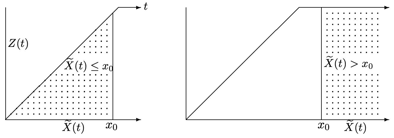
We do this first for the example of the distribution function of duration, \(\operatorname{Pr}\left\{\widetilde{X}(t) \leq x_{0}\right\}\), where we first assume that \(x_{0} \leq t\). As illustrated in Figure 4.19, the corresponding reward function \(R(t)\) is 1 in the triangular region where \(\tilde{X}(t) \leq x_{0}\) and \(Z(t)<\tilde{X}(t)\). It is 0 elsewhere.

Figure 4.19: Finding \(\mathrm{F}_{\widetilde{X}(t)}\left(x_{0}\right)\) for \(x_{0} \leq t\) and for \(x_{0}>t\).

\[\begin{aligned}
\operatorname{Pr}\left\{\tilde{X}(t) \leq x_{0}\right\} &=\int_{z=0}^{x_{0}} \int_{x=z}^{x_{0}} m^{\prime}(t-z) \mathrm{f}_{X}(x) d x d z \\
&=\int_{z=0}^{x_{0}} m^{\prime}(t-z)\left[\mathrm{F}_{X}\left(x_{0}\right)-\mathrm{F}_{X}(z)\right] d z \\
&=\mathrm{F}_{X}\left(x_{0}\right)\left[m(t)-m\left(t-x_{0}\right)\right]-\int_{t-x_{0}}^{t} \mathrm{~F}_{X}(t-\tau) d m(\tau)
\end{aligned}\label{4.92} \]

For the opposite case, where \(x_{0}>t\), it is easier to find \(\operatorname{Pr}\left\{\tilde{X}(t)>x_{0}\right\}\). As shown in the figure, this is the region where \(0 \leq Z(t) \leq t\) and \(\tilde{X}(t)>x_{0}\). There is a subtlety here in that the incremental areas we are using are only valid for \(Z(t)<t\). If the age is equal to \(t\), then no renewals have occured in \((0, t]\), so that \(\operatorname{Pr}\left\{\tilde{X}(t)>x_{0} ; Z(t)=t\right\}=\mathrm{F}_{X}^{c}\left(x_{0}\right)\). Thus

\[\begin{aligned}
\operatorname{Pr}\left\{\tilde{X}(t)>x_{0}\right\} &=\mathrm{F}_{X}^{c}\left(x_{0}\right)+\int_{z=0}^{t^{-}} \int_{x=x_{0}}^{\infty} m^{\prime}(t-z) \mathrm{f}_{X}(x) d x d z \\
&=\mathrm{F}_{X}^{c}\left(x_{0}\right)+m(t) \mathrm{F}_{X}^{c}\left(x_{0}\right)
\end{aligned}\label{4.93} \]

As a sanity test, the renewal equation, (4.53), can be used to show that the sum of \ref{4.92} and \ref{4.93} at \(x_{0}=t\) is equal to 1 (as they must be if the equations are correct).

We can now take the limit, \(\lim _{t \rightarrow \infty} \operatorname{Pr}\left\{\tilde{X}(t) \leq x_{0}\right\}\). For any given \(x_{0}\), \ref{4.92} holds for sufficiently large \(t\), and the key renewal theorem can be used since the integral has a finite range. Thus,

\[\begin{aligned}
\lim _{t \rightarrow \infty} \operatorname{Pr}\left\{\tilde{X}(t) \leq x_{0}\right\} &=\frac{1}{\overline{X}}\left[x_{0} \mathrm{~F}_{X}\left(x_{0}\right)-\int_{0}^{x_{0}} \mathrm{~F}_{X}(x) d x\right] \\
&=\frac{1}{\overline{X}} \int_{0}^{x_{0}}\left[\mathrm{~F}_{X}\left(x_{0}\right)-\mathrm{F}_{X}(x)\right] d x \\
&=\frac{1}{\overline{X}} \int_{0}^{x_{0}}\left[\mathrm{~F}_{X}^{c}(x)-d F_{X}^{c}\left(x_{0}\right)\right] d x
\end{aligned}\label{4.94} \]

It is easy to see that the right side of \ref{4.94} is increasing from 0 to 1 with increasing \(x_{0}\), i.e., it is a distribution function.

After this example, it is now straightforward to write down the expected value of an arbitrary renewal-reward function \(R(t)\) whose sample value at \(Z(t)=z\) and \(X(t)=x\) is denoted by \(\mathcal{R}(z, x)\). We have

\[\mathrm{E}[R(t)]=\int_{x=t}^{\infty} \mathcal{R}(t, x) d \mathrm{~F}_{X}(x)+\int_{z=0}^{t} \int_{x=z}^{\infty} \mathcal{R}(z, x) d \mathrm{~F}_{X}(x) d m(t-z)\label{4.95} \]

The first term above arises from the subtlety discussed above for the case where \(Z(t)=t\). The second term is simply the integral over the semi-infinite trapezoidal area in Figure 4.19.

The analysis up to this point applies to both the arithmetic and nonarithmetic cases, but we now must assume again that the renewal process is nonarithmetic. If the inner integral, i.e., \(\int_{x=z}^{\infty} \mathcal{R}(z, x) d \mathrm{~F}_{X}(x)\), as a function of \(z\), is directly Riemann integrable, then not only can the key renewal theorem be applied to this second term, but also the first term must approach 0 as \(t \rightarrow \infty\). Thus the limit of \ref{4.95} as \(t \rightarrow \infty\) is

\[\lim _{t \rightarrow \infty} \mathrm{E}[R(t)]=\frac{1}{\overline{X}} \int_{z=0}^{\infty} \int_{x=z}^{\infty} \mathcal{R}(z, x) d \mathrm{~F}_{X}(x) d z\label{4.96} \]

This is the same expression as found for the time-average renewal reward in Theorem 4.4.1. Thus, as indicated earlier, we can now equate any time-average result for the nonarithmetic case with the corresponding limiting ensemble average, and the same equations have been derived in both cases.

As a simple example of (4.96), let \(\mathcal{R}(z, t)=x\). Then \(\mathrm{E}[R(t)]=\mathrm{E}[\tilde{X}(t)]\) and

\[\begin{aligned}
\lim _{t \rightarrow \infty} \mathrm{E}[\tilde{X}(t)] &=\frac{1}{\overline{X}} \int_{z=0}^{\infty} \int_{x=z}^{\infty} x d \mathrm{~F}_{X}(x) d z=\int_{x=0}^{\infty} \int_{z=0}^{x} x d z d \mathrm{~F}_{X}(x) \\
&=\frac{1}{\overline{X}} \int_{x=0}^{\infty} x^{2} d \mathrm{~F}_{X}(x)=\frac{\mathrm{E}\left[X^{2}\right]}{\overline{X}}
\end{aligned}\label{4.97} \]

After calculating the integral above by interchanging the order of integration, we can go back and assert that the key renewal theorem applies if \(\mathrm{E}\left[X^{2}\right]\) is finite. If it is infinite, then it is not hard to see that \(\lim _{t \rightarrow \infty} \mathrm{E}[\tilde{X}(t)]\) is infinite also.

It has been important, and theoretically reassuring, to be able to find ensemble-averages for nonarithmetic renewal-reward functions in the limit of large \(t\) and to show (not surprisingly) that they are the same as the time-average results. The ensemble-average results are quite tricky, though, and it is wise to check results achieved that way with the corresponding time-average results.

---

²¹This must seem like mathematical nitpicking to many readers. However, \(m(t)\) is the expected number of renewals in \((0, t]\), and how \(m(t)\) varies with \(t\), is central to this chapter and keeps reappearing.

²²Finding the limiting expectations from the limiting PMF’s requires interchanging a limit with an expectation. This can be justified (in both \ref{4.70} and (4.71)) by assuming that \(X\) has a finite second moment and noting that all the terms involved are positive, that \(\operatorname{Pr}\{\text { arrival at } j\} \leq 1\) for all \(j\), and that \(\mathrm{p}_{X}(k) \leq 1\) for all \(k\).

²³This seems to be rather abstract mathematics, but as engineers, we often evaluate functions with step discontinuities by ignoring the values at the discontinuities or evaluating these points by adhoc means.