4.10: Exercises

Exercise 4.1

The purpose of this exercise is to show that for an arbitrary renewal process, \(N(t)\), the number of renewals in \((0, t]\) is a (non-defective) random variable.

1. Let \(X_{1}, X_{2}, \ldots\), be a sequence of IID inter-renewal rv’s. Let \(S_{n}=X_{1}+\cdots+X_{n}\) be the corresponding renewal epochs for each \(n \geq 1\). Assume that each \(X_{i}\) has a finite expectation \(\overline{X}>0\) and, for any given \(t > 0\), use the weak law of large numbers to show that \(\lim _{n \rightarrow \infty} \operatorname{Pr}\left\{S_{n} \leq t\right\}=0\).
2. Use part a) to show that \(\lim _{n \rightarrow \infty} \operatorname{Pr}\{N \geq n\}=0\) and explain why this means that \(N(t)\) is a rv, i.e., is not defective.
3. Now suppose that the \(X_{i}\) do not have a finite mean. Consider truncating each \(X_{i}\) to \(\breve{X}_{i}\), where for any given \(b>0\), \(\breve{X}_{i}=\min \left(X_{i}, b\right)\). Let \(\breve{N}(t)\) be the renewal counting process for the inter-renewal intervals \(\breve{X}_{i}\). Show that \(\breve{N}(t)\) is non-defective for each \(t > 0\). Show that \(N(t) \leq \breve{N}(t)\) and thus that \(N(t)\) is non-defective. Note: Large inter-renewal intervals create small values of \(N(t)\), and thus \(\mathrm{E}[X]=\infty\) has nothing to do with potentially large values of \(N(t)\), so the argument here was purely technical.

Exercise 4.2

The purpose of this exercise is to show that, for an arbitrary renewal process, \(N(t)\), the number of renewals in \((0, t]\), has finite expectation.

1. Let the inter-renewal intervals have the distribution \(\mathrm{F}_{X}(x)\), with, as usual, \(\mathrm{F}_{X}(0)=0\). Using whatever combination of mathematics and common sense is comfortable for you, show that numbers \(\epsilon>0\) and \(\delta>0\) must exist such that \(\mathrm{F}_{X}(\delta) \leq 1-\epsilon\). In other words, you are to show that a positive rv must take on some range of of values bounded away from zero with positive probability.
2. Show that \(\operatorname{Pr}\left\{S_{n} \leq \delta\right\} \leq(1-\epsilon)^{n}\).
3. Show that \(\mathrm{E}[N(\delta)] \leq 1 / \epsilon\).
4. Show that for every integer \(k\), \(\mathrm{E}[N(k \delta)] \leq k / \epsilon\) and thus that \(\mathrm{E}[N(t)] \leq \frac{t+\delta}{\epsilon \delta}\) for any \(t > 0\).
5. Use your result here to show that \(N(t)\) is non-defective.

Exercise 4.3

Let \(\left\{X_{i} ; i \geq 1\right\}\) be the inter-renewal intervals of a renewal process generalized to allow for inter-renewal intervals of size 0 and let \(\operatorname{Pr}\left\{X_{i}=0\right\}=\alpha\), \(0<\alpha<1\). Let \(\left\{Y_{i} ; i \geq 1\right\}\) be the sequence of non-zero interarrival intervals. For example, if \(X_1=x_{1}>0, X_{2}=0, X_{3}=x_{3}>0, \ldots\), then \(Y_{1}=x_{1}, Y_{2}=x_{3}, \ldots,.\)

1. Find the distribution function of each \(Y_{i}\) in terms of that of the \(X_{i}\).
2. Find the PMF of the number of arrivals of the generalized renewal process at each epoch at which arrivals occur.
3. Explain how to view the generalized renewal process as an ordinary renewal process with inter-renewal intervals \(\left\{Y_{i} ; i \geq 1\right\}\) and bulk arrivals at each renewal epoch.
4. When a generalized renewal process is viewed as an ordinary renewal process with bulk arrivals, what is the distribution of the bulk arrivals? (The point of this part is to illustrate that bulk arrivals on an ordinary renewal process are considerably more general than generalized renewal processes.)

Exercise 4.4

Is it true for a renewal process that:

1. \(N(t)<n\) if and only if \(S_{n}>t\)?
2. \(N(t) \leq n\) if and only if \(S_{n} \geq t\)?
3. \(N(t)>n\) if and only if \(S_{n}<t\)?

Exercise 4.5

(This shows that convergence WP1 implies convergence in probability.) Let \(\left\{Y_{n} ; n \geq 1\right\}\) be a sequence of rv’s that converges to 0 WP1. For any positive integers \(m\) and \(k\), let

\(A(m, k)=\left\{\omega:\left|Y_{n}(\omega)\right| \leq 1 / k \quad \text { for all } n \geq m\right\}\)

1. Show that if \(\lim _{n \rightarrow \infty} Y_{n}(\omega)=0\) for some given \(\omega\), then (for any given \(k\)) \(\omega \in A(m, k)\) for some positive integer \(m\).
2. Show that for all \(k \geq 1\)

   \(\operatorname{Pr}\left\{\bigcup_{m=1}^{\infty} A(m, k)\right\}=1\)

3. Show that, for all \(m \geq 1\), \(A(m, k) \subseteq A(m+1, k)\). Use this (plus (1.9)) to show that

   \(\lim _{m \rightarrow \infty} \operatorname{Pr}\{A(m, k)\}=1\)

4. Show that if \(\omega \in A(m, k)\), then \(\left|Y_{m}(\omega)\right| \leq 1 / k\). Use this (plus part c) to show that

   \(\lim _{m \rightarrow \infty} \operatorname{Pr}\left\{\left|Y_{m}\right|>1 / k\right\}=0\)

Since \(k \geq 1\) is arbitrary, this shows that \(\left\{Y_{n} ; n \geq 1\right\}\) converges in probabiity.

Exercise 4.6

In this exercise, we find an explicit expression for \(\left\{\omega: \lim _{n} Y_{n}=0\right\}\). You may use whatever level of mathematical precision you feel comfortable with.

1. Let \(\left\{Y_{n} ; n \geq 1\right\}\) be a sequence of rv’s. Using the definition of convergence for a sequence of numbers, justify the following set equivalences:

   \(\begin{aligned}
   \left\{\omega: \lim _{n} Y_{n}(\omega)=0\right\} &=\bigcap_{k=1}^{\infty}\left\{\omega: \text { there exists an } m \text { such that }\left|Y_{n}(\omega)\right| \leq 1 / k \text { for all } n \geq m\right\} \\
   &=\bigcap_{k=1}^{\infty} \bigcup_{m=1}^{\infty}\left\{\omega: Y_{n}(\omega) \leq 1 / k \text { for all } n \geq m\right\} \\
   &=\bigcap_{k=1}^{\infty} \bigcup_{m=1}^{\infty} \bigcap_{n=m}^{\infty}\left\{\omega: Y_{n}(\omega) \leq 1 / k\right\}
   \end{aligned}\)

2. Explain how this shows that \(\left\{\omega: \lim _{n} Y_{n}(\omega)=0\right\}\) must be an event.
3. Use deMorgan’s laws to show that the complement of the above equivalence is

   \(\left\{\omega: \lim _{n} Y_{n}(\omega)=0\right\}^{c}=\bigcup_{k=1}^{\infty} \bigcap_{m=1}^{\infty} \bigcup_{n=m}^{\infty}\left\{\omega: Y_{n}(\omega)>1 / k\right\}\)

4. Show that for \(\left\{Y_{n} ; n \geq 1\right\}\) to converge WP1, it is necessary and sufficient to satisfy

   \(\operatorname{Pr}\left\{\bigcap_{m=1}^{\infty} \bigcup_{n=m}^{\infty}\left\{Y_{n}>1 / k\right\}\right\}=0 \quad \text { for all } k \geq 1\)

5. Show that for \(\left\{Y_{n} ; n \geq 1\right\}\) to converge WP1, it is necessary and sufficient to satisfy

   \(\lim _{m \rightarrow \infty} \operatorname{Pr}\left\{\bigcup_{n=m}^{\infty}\left\{Y_{n}>1 / k\right\}\right\}=0 \quad \text { for all } k \geq 1\)

Hint: Use part a) of Exercise 4.7. Note: Part e) provides an equivalent condition that is often useful in establishing convergence WP1. It also brings out quite clearly the difference between convergence WP1 and convergence in probability.

Exercise 4.7

Consider the event \(\bigcap_{m \geq 1} \bigcup_{n \geq m} A_{n}\) where \(A_{1}, A_{2}, \ldots\), are arbitrary events.

1. Show that

   \(\lim _{m \rightarrow \infty} \operatorname{Pr}\left\{\bigcup_{n \geq m} A_{n}\right\}=0 \quad \Longleftrightarrow \quad \operatorname{Pr}\left\{\bigcap_{m \geq 1} \bigcup_{n \geq m} A_{n}\right\}=0\)

   Hint: Apply the complement of (1.9).

2. Show that if \(\sum_{m=1}^{\infty} \operatorname{Pr}\left\{A_{m}\right\}<\infty\), then \(\operatorname{Pr}\left\{\bigcap_{m} \bigcup_{n \geq m} A_{n}\right\}=0\). Hint: Recall that if \(\sum_{m=1}^{\infty} \operatorname{Pr}\left\{A_{m}\right\}<\infty\), then \(\lim _{m \rightarrow \infty} \operatorname{Pr}\left\{\bigcup_{n \geq m} A_{n}\right\}=0\). Combine this with a). This well-known result is called the Borel-Cantelli lemma.
3. The set \(\operatorname{Pr}\left\{\bigcap_{m} \bigcup_{n \geq m} A_{n}\right\}\) is often referred to as the set of ω that are contained in infinitely many of the \(A_{n}\). Without trying to be precise about what this latter statement means, explain why it is a good way to think about \(\operatorname{Pr}\left\{\bigcap_{m} \bigcup_{n \geq m} A_{n}\right\}\). Hint: Consider an ω that is contained in some finite number \(k\) of the sets \(A_{n}\) and argue that there must be an integer \(m\) such that \(\omega \notin A_{n}\) for all \(n>m\).

Exercise 4.8

Let \(\left\{X_{i} ; i \geq 1\right\}\) be the inter-renewal intervals of a renewal process and assume that \(\mathrm{E}\left[X_{i}\right]=\infty\). Let \(b>0\) be an arbitrary number and \(\breve{X}_{i}\) be a truncated random variable defined by \(\breve{X}_{i}=X_{i}\) if \(X_{i} \leq b\) and \(\breve{X}_{i}=b\) otherwise.

1. Show that for any constant \(M>0\), there is a \(b\) sufficiently large so that \(\mathrm{E}\left[\breve{X}_{i}\right] \geq M\).
2. Let \(\{\breve{N}(t) ; t \geq 0\}\) be the renewal counting process with inter-renewal intervals \(\left\{\breve{X}_{i} ; i \geq 1\right\}\) and show that for all \(t>0\), \(\breve{N}(t) \geq N(t)\).
3. Show that for all sample functions \(N(t, \omega)\), except a set of probability 0, \(N(t, \omega) / t<2 / M\) for all sufficiently large t. Note: Since \(M\) is arbitrary, this means that \(\lim N(t) / t=0\) with probability 1.

Exercise 4.9

Let \(Y(t)=S_{N(t)+1}-t\) be the residual life at time t of a renewal process. First consider a renewal process in which the interarrival time has density \(\mathrm{f}_{X}(x)=e^{-x} ; x \geq 0\), and next consider a renewal process with density

\(\mathrm{f}_{X}(x)=\frac{3}{(x+1)^{4}} ; \quad x \geq 0\)

For each of the above densities, use renewal-reward theory to find:

1. the time-average of \(Y(t)\)
2. the second moment in time of \(Y(t)\) (i.e., \(\lim _{T \rightarrow \infty} \frac{1}{T} \int_{0}^{T} Y^{2}(t) d t\))

For the exponential density, verify your answers by finding \(\mathrm{E}[Y(t)]\) and \(\mathrm{E}\left[Y^{2}(t)\right]\) directly.

Exercise 4.10

Consider a variation of an M/G/1 queueing system in which there is no facility to save waiting customers. Assume customers arrive according to a Poisson process of rate \(\lambda\). If the server is busy, the customer departs and is lost forever; if the server is not busy, the customer enters service with a service time distribution function denoted by \(\mathrm{F}_{Y}(y)\).

Successive service times (for those customers that are served) are IID and independent of arrival times. Assume that customer number 0 arrives and enters service at time \(t=0\).

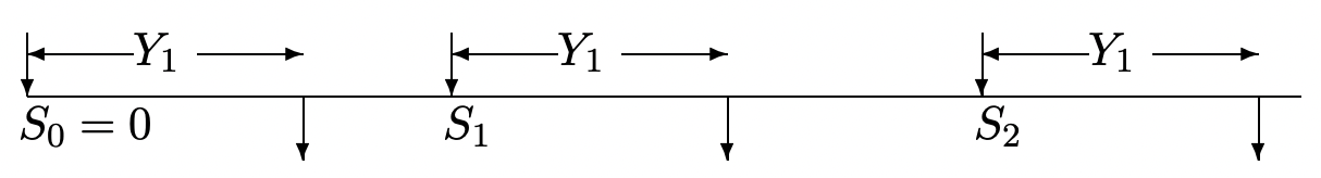
1. Show that the sequence of times \(S_{1}, S_{2}, \ldots\) at which successive customers enter service are the renewal times of a renewal process. Show that each inter-renewal interval \(X_{i}=S_{i}-S_{i-1}\) (where \(S_{0}=0\)) is the sum of two independent random variables, \(Y_{i}+U_{i}\) where \(Y_{i}\) is the \(i\)th service time; find the probability density of \(U_{i}\).
2. Assume that a reward (actually a cost in this case) of one unit is incurred for each customer turned away. Sketch the expected reward function as a function of time for the sample function of inter-renewal intervals and service intervals shown below; the expectation is to be taken over those (unshown) arrivals of customers that must be turned away.

   

3. Let \(\int_{0}^{t} R(\tau) d \tau\) denote the accumulated reward (i.e., cost) from 0 to \(t\) and find the limit as \(t \rightarrow \infty\) of \((1 / t) \int_{0}^{t} R(\tau) d \tau\). Explain (without any attempt to be rigorous or formal) why this limit exists with probability 1.
4. In the limit of large \(t\), find the expected reward from time \(t\) until the next renewal. Hint: Sketch this expected reward as a function of \(t\) for a given sample of inter-renewal intervals and service intervals; then find the time-average.
5. Now assume that the arrivals are deterministic, with the first arrival at time 0 and the \(n\)th arrival at time \(n-1\). Does the sequence of times \(S_{1}, S_{2}, \ldots\) at which subsequent customers start service still constitute the renewal times of a renewal process? Draw a sketch of arrivals, departures, and service time intervals. Again find \(\lim _{t \rightarrow \infty}\left(\int_{0}^{t} R(\tau) d \tau\right) / t\).

Exercise 4.11

Let \(Z(t)=t-S_{N(t)}\) be the age of a renewal process and \(Y(t)=S_{N(t)+1}-t\) be the residual life. Let \(\mathrm{F}_{X}(x)\) be the distribution function of the inter-renewal interval and find the following as a function of \(\mathrm{F}_{X}(x)\):

1. \(\operatorname{Pr}\{Y(t)>x \mid Z(t)=s\}\)
2. \(\operatorname{Pr}\{Y(t)>x \mid Z(t+x / 2)=s\}\)
3. \(\operatorname{Pr}\{Y(t)>x \mid Z(t+x)>s\}\) for a Poisson process.

Exercise 4.12

Let \(\mathrm{F}_{Z}(z)\) be the fraction of time (over the limiting interval \((0, \infty)\) that the age of a renewal process is at most \(z\). Show that \(\mathrm{F}_{Z}(z)\) satisfies

\(\mathrm{F}_{Z}(z)=\frac{1}{\overline{X}} \int_{x=0}^{y} \operatorname{Pr}\{X>x\} d x \quad \text { WP1 }\)

Hint: Follow the argument in Example 4.4.5.

Exercise 4.13

1. Let \(J\) be a stopping rule and \(\mathbb{I}_{\{J \geq n\}}\) be the indicator random variable of the event \(\{J \geq n\}\). Show that \(J=\sum_{n \geq 1} \mathbb{I}_{\{J \geq n}\).
2. Show that \(\mathbb{I}_{J \geq 1} \geq \mathbb{I}_{J \geq 2} \geq \ldots\), i.e., show that for each \(n>1, \mathbb{I}_{J \geq n}(\omega) \geq \mathbb{I}_{J \geq n+1}(\omega)\) for each \(\omega \in \Omega\) (except perhaps for a set of probability 0).

Exercise 4.14

1. Use Wald’s equality to compute the expected number of trials of a Bernoulli process up to and including the \(k\)th success.
2. Use elementary means to find the expected number of trials up to and including the first success. Use this to find the expected number of trials up to and including the \(k\)th success. Compare with part a).

Exercise 4.15

A gambler with an initial finite capital of \(d>0\) dollars starts to play a dollar slot machine. At each play, either his dollar is lost or is returned with some additional number of dollars. Let \(X_{i}\) be his change of capital on the \(i\)th play. Assume that \(\left\{X_{i} ; i=1,2, \ldots\right\}\) is a set of IID random variables taking on integer values {−1, 0, 1, . . . }. Assume that \(\mathrm{E}\left[X_{i}\right]<0\). The gambler plays until losing all his money (i.e., the initial \(d\) dollars plus subsequent winnings).

1. Let \(J\) be the number of plays until the gambler loses all his money. Is the weak law of large numbers sufficient to argue that \(\lim _{n \rightarrow \infty} \operatorname{Pr}\{J>n\}=0\) (i.e., that \(J\) is a random variable) or is the strong law necessary?
2. Find \(\mathrm{E}[J]\). Hint: The fact that there is only one possible negative outcome is important here.

Exercise 4.16

Let \(\left\{X_{i} ; i \geq 1\right\}\) be IID binary random variables with \(P_{X}(0)=P_{X}(1)=1/2\). Let \(J\) be a positive integer-valued random variable defined on the above sample space of binary sequences and let \(S_{J}=\sum_{i=1}^{J} X_{i}\). Find the simplest example you can in which \(J\) is not a stopping trial for \(\left\{X_{i} ; i \geq 1\right\}\) and where \(\mathrm{E}[X] \mathrm{E}[J] \neq \mathrm{E}\left[S_{J}\right]\). Hint: Try letting \(J\) take on only the values 1 and 2.

Exercise 4.17

Let \(J=\min \left\{n \mid S_{n} \leq b \text { or } S_{n} \geq a\right\}\), where \(a\) is a positive integer, \(b\) is a negative integer, and \(S_{n}=X_{1}+X_{2}+\cdots+X_{n}\). Assume that \(\left\{X_{i} ; i \geq 1\right\}\) is a set of zero mean IID rv’s that can take on only the set of values {−1, 0, +1}, each with positive probability.

1. Is \(J\) a stopping rule? Why or why not? Hint: The more difficult part of this is to argue that \(J\) is a random variable (i.e., non-defective); you do not need to construct a proof of this, but try to argue why it must be true.
2. What are the possible values of \(S_{J}\)?
3. Find an expression for \(\mathrm{E}\left[S_{J}\right]\) in terms of \(p, a\), and \(b\), where \(p=\operatorname{Pr}\left\{S_{J} \geq a\right\}\).
4. Find an expression for \(\mathrm{E}\left[S_{J}\right]\) from Wald’s equality. Use this to solve for \(p\).

Exercise 4.18

Show that the interchange of expectation and sum in \ref{4.32} is valid if \(\mathrm{E}[J]<\infty\). Hint: First express the sum as \(\sum_{n=1}^{k-1} X_{n} \mathbb{I}_{J \geq n}+\sum_{n=k}^{\infty}\left(X_{n}^{+}+X_{n}^{-}\right) \mathbb{I}_{J \geq n}\) and then consider the limit as \(k \rightarrow \infty\).

Exercise 4.19

Consider an amnesic miner trapped in a room that contains three doors. Door 1 leads him to freedom after two-day’s travel; door 2 returns him to his room after four-day’s travel; and door 3 returns him to his room after eight-day’s travel. Suppose each door is equally likely to be chosen whenever he is in the room, and let \(T\) denote the time it takes the miner to become free.

1. Define a sequence of independent and identically distributed random variables \(X_{1}, X_{2}, \ldots\) and a stopping rule \(J\) such that

   \(T=\sum_{i=1}^{J} X_{i}\).

2. Use Wald’s equality to find \(\mathrm{E}[T]\).
3. Compute \(\mathrm{E}\left[\sum_{i=1}^{J} X_{i} \mid J=n\right]\) and show that it is not equal to \(\mathrm{E}\left[\sum_{i=1}^{n} X_{i}\right]\).
4. Use part c) for a second derivation of \(\mathrm{E}[T]\).

Exercise 4.20

1. Consider a renewal process for which the inter-renewal intervals have the PMF \(p_{X}(1)=p_{X}(2)=1 / 2\). Use elementary combinatorics to show that \(m(1)=1 / 2\), \(m(2)=5 / 4\), and \(m(3)=15 / 8\).
2. Use elementary means to show that \(\mathrm{E}\left[S_{N(1)}\right]=1 / 2\) and \(\mathrm{E}\left[S_{N(1)+1}\right]=9 / 4\). Verify \ref{4.35} in this case (i.e., for \(t=1\)) and show that \(N(1)\) is not a stopping trial. Note also that the expected duration, \(\mathrm{E}\left[S_{N(1)+1}-S_{N(1)}\right]\) is not equal to \(\overline{X}\).
3. Consider a more general form of part a) where \(\operatorname{Pr}\{X=1\}=1-p\) and \(\operatorname{Pr}\{X=2\}=p\). Let \(\operatorname{Pr}\left\{W_{n}=1\right\}=x_{n}\) and show that \(x_{n}\) satisfies the difference equation \(x_{n}=1-p x_{n-1}\) for \(n \geq 1\) where by convention \(x_{0}=1\). Use this to show that

   \[x_{n}=\frac{1-(-p)^{n+1}}{1+p}\label{4.112} \]

   From this, solve for \(m(n)\) for \(n \geq 1\).

Exercise 4.21

Let \(\{N(t) ; t>0\}\) be a renewal counting process generalized to allow for inter-renewal intervals \(\left\{X_{i}\right\}\) of duration 0. Let each \(X_{i}\) have the PMF \(\operatorname{Pr}\left\{X_{i}=0\right\}=1-\epsilon\); \(\operatorname{Pr}\left\{X_{i}=1 / \epsilon\right\}=\epsilon\).

1. Sketch a typical sample function of \(\{N(t) ; t>0\}\). Note that \(N(0)\) can be non-zero (i.e., \(N(0)\) is the number of zero interarrival times that occur before the first non-zero interarrival time).
2. Evaluate \(\mathrm{E}[N(t)]\) as a function of \(t\).
3. Sketch \(\mathrm{E}[N(t)] / t\) as a function of \(t\).
4. Evaluate \(\mathrm{E}\left[S_{N(t)+1}\right]\) as a function of \(t\) (do this directly, and then use Wald’s equality as a check on your work).
5. Sketch the lower bound \(\mathrm{E}[N(t)] / t \geq 1 / \mathrm{E}[X]-1 / t\) on the same graph with part c).
6. Sketch \(\mathrm{E}\left[S_{N(t)+1}-t\right]\) as a function of \(t\) and find the time average of this quantity.
7. Evaluate \(\mathrm{E}\left[S_{N(t)}\right]\) as a function of t; verify that \(\mathrm{E}\left[S_{N(t)}\right] \neq \mathrm{E}[X] \mathrm{E}[N(t)]\).

Exercise 4.22

Let \(\{N(t) ; t>0\}\) be a renewal counting process and let \(m(t)=\mathrm{E}[N(t)]\) be the expected number of arrivals up to and including time \(t\). Let \(\left\{X_{i} ; i \geq 1\right\}\) be the inter-renewal times and assume that \(\mathrm{F}_{X}(0)=0\).

1. For all \(x>0\) and \(t>x\) show that \(\mathrm{E}\left[N(t) \mid X_{1}=x\right]=\mathrm{E}[N(t-x)]+1\).
2. Use part a) to show that \(m(t)=\mathrm{F}_{X}(t)+\int_{0}^{t} m(t-x) d \mathrm{~F}_{X}(x)\) for \(t>0\). This equation is the renewal equation derived differently in (4.52).
3. Suppose that \(X\) is an exponential random variable of parameter \(\lambda\). Evaluate \(L_{m}(s)\) from (4.54); verify that the inverse Laplace transform is \(\lambda t\); \(t \geq 0\).

Exercise 4.23

1. Let the inter-renewal interval of a renewal process have a second order Erlang density, \(f_{X}(x)=\lambda^{2} x \exp (-\lambda x)\). Evaluate the Laplace transform of \(m(t)=\mathrm{E}[N(t)]\).
2. Use this to evaluate \(m(t)\) for \(t \geq 0\). Verify that your answer agrees with (4.56).
3. Evaluate the slope of \(m(t)\) at \(t=0\) and explain why that slope is not surprising.
4. View the renewals here as being the even numbered arrivals in a Poisson process of rate \(\lambda\). Sketch \(m(t)\) for the process here and show one half the expected number of arrivals for the Poisson process on the same sketch. Explain the difference between the two.

Exercise 4.24

1. Let \(N(t)\) be the number of arrivals in the interval \((0, t]\) for a Poisson process of rate \(\lambda\). Show that the probability that \(N(t)\) is even is \([1+\exp (-2 \lambda t)] / 2\). Hint: Look at the power series expansion of \(\exp (-\lambda t)\) and that of \(\exp (\lambda t)\), and look at the sum of the two. Compare this with \(\sum_{n \text { even }} \operatorname{Pr}\{N(t)=n\}\)
2. Let \(\tilde{N}(t)\) be the number of even numbered arrivals in \((0, t]\). Show that \(\tilde{N}(t)=N(t) / 2-\mathbb{I}_{\text {odd }}(t) / 2 \text { where } \mathbb{I}_{\text {odd }}(t)\) is a random variable that is 1 if \(N(t)\) is odd and 0 otherwise.
3. Use parts a) and b) to find \(\mathrm{E}[\tilde{N}(t)]\). Note that this is \(m(t)\) for a renewal process with 2nd order Erlang inter-renewal intervals.

Exercise 4.25

1. Consider a function \(r(z) \geq 0\) defined as follows for \(0 \leq z<\infty\): For each integer \(n \geq 1\) and each integer \(k\), \(1 \leq k<n, r(z)=1\) for \(n+k / n \leq z \leq n+k / n+2^{-n}\). For all other \(z\), \(r(z)=0\). Sketch this function and show that \(r(z)\) is not directly Riemann integrable.
2. Evaluate the Riemann integral \(\int_{0}^{\infty} r(z) d z\).
3. Suppose \(r(z)\) is decreasing, i.e., that \(r(z) \geq r(y)\) for all \(y>z>0\). Show tht if \(r(z)\) is Riemann integrable, it is also directly Riemann integrable.
4. Suppose \(f(z) \geq 0\), defined for \(z \geq 0\), is decreasing and Riemann integrable and that \(f(z) \geq r(z)\) for all \(z \geq 0\). Show that \(r(z)\) is Directly Riemann integrable.
5. Let \(X\) be a non-negative rv for which \(\mathrm{E}\left[X^{2}\right]<\infty\). Show that \(x \mathrm{~F}_{X}^{\mathrm{c}}(x)\) is directly Riemann integrable. Hint: Consider \(y \mathrm{~F}_{X}^{\mathrm{c}}(y)+\int_{y}^{\infty} \mathrm{F}_{X}(x) d x\) and use Figure 1.7 (or use integration by parts) to show that this expression is decreasing in \(y\).

Exercise 4.26

Let \(Z(t), Y(t), \widetilde{X}(t)\) denote the age, residual life, and duration at time \(t\) for a renewal counting process \(\{N(t) ; t>0\}\) in which the interarrival time has a density given by \(f(x)\). Find the following probability densities; assume steady state.

1. \(\mathrm{f}_{Y(t)}(y \mid Z(t+s / 2)=s)\) for given \(s>0\).
2. \(\mathrm{f}_{Y(t), Z(t)}(y, z)\).
3. \(\mathrm{f}_{Y(t)}(y \mid \widetilde{X}(t)=x)\).
4. \(\mathrm{f}_{Z(t)}(z \mid Y(t-s / 2)=s)\) for given \(s>0\).
5. \(\mathrm{f}_{Y(t)}(y \mid Z(t+s / 2) \geq s)\) for given \(s>0\).

Exercise 4.27

1. Find \(\lim _{t \rightarrow \infty}\{\mathrm{E}[N(t)]-t / \overline{X}\}\) for a renewal counting process \(\{N(t) ; t>0\}\) with inter-renewal times \(\left\{X_{i} ; i \geq 1\right\}\). Hint: use Wald’s equation.
2. Evaluate your result for the case in which \(X\) is an exponential random variable (you already know what the result should be in this case).
3. Evaluate your result for a case in which \(\mathrm{E}[X]<\infty\) and \(\mathrm{E}\left[X^{2}\right]=\infty\). Explain (very briefly) why this does not contradict the elementary renewal theorem.

Exercise 4.28

Customers arrive at a bus stop according to a Poisson process of rate \(\lambda\). Independently, buses arrive according to a renewal process with the inter-renewal interval distribution \(\mathrm{F}_{X}(x)\). At the epoch of a bus arrival, all waiting passengers enter the bus and the bus leaves immediately. Let \(R(t)\) be the number of customers waiting at time \(t\).

1. Draw a sketch of a sample function of \(R(t)\).
2. Given that the first bus arrives at time \(X_{1}=x\), find the expected number of customers picked up; then find \(\mathrm{E}\left[\int_{0}^{x} R(t) d t\right]\), again given the first bus arrival at \(X_{1}=x\).
3. Find \(\lim _{t \rightarrow \infty} \frac{1}{t} \int_{0}^{t} R(\tau) d \tau\) (with probability 1). Assuming that \(\mathrm{F}_{X}\) is a non-arithmetic distribution, find \(\lim _{t \rightarrow \infty} \mathrm{E}[R(t)]\). Interpret what these quantities mean.
4. Use part c) to find the time-average expected wait per customer.
5. Find the fraction of time that there are no customers at the bus stop. (Hint: this part is independent of a), b), and c); check your answer for \(\mathrm{E}[X] \ll 1 / \lambda\)).

Exercise 4.29

Consider the same setup as in Exercise 4.28 except that now customers arrive according to a non-arithmetic renewal process independent of the bus arrival process. Let \(1 / \lambda\) be the expected inter-renewal interval for the customer renewal process. Assume that both renewal processes are in steady state (i.e., either we look only at \(t \gg 0\), or we assume that they are equilibrium processes). Given that the nth customer arrives at time \(t\), find the expected wait for customer \(n\). Find the expected wait for customer \(n\) without conditioning on the arrival time.

Exercise 4.30

Let \(\left\{N_{1}(t) ; t>0\right\}\) be a Poisson counting process of rate \(\lambda\). Assume that the arrivals from this process are switched on and off by arrivals from a non-arithmetic renewal counting process \(\left\{N_{2}(t) ; t>0\right\}\) (see figure below). The two processes are independent.

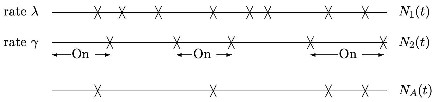
Let \(\left\{N_{A}(t) ; t \geq 0\right\}\) be the switched process; that is \(N_{A}(t)\) includes arrivals from \(\{N_{1}(t) ; t>0\}\) while \(N_{2}(t)\) is even and excludes arrivals from \(\left\{N_{1}(t) ; t>0\right\}\) while \(N_{2}(t)\) is odd.

1. Is \(N_{A}(t)\) a renewal counting process? Explain your answer and if you are not sure, look at several examples for \(N_{2}(t)\).
2. Find \(\lim _{t \rightarrow \infty} \frac{1}{t} N_{A}(t)\) and explain why the limit exists with probability 1. Hint: Use symmetry—that is, look at \(N_{1}(t)-N_{A}(t)\). To show why the limit exists, use the renewalreward theorem. What is the appropriate renewal process to use here?
3. Now suppose that \(\left\{N_{1}(t) ; t>0\right\}\) is a non-arithmetic renewal counting process but not a Poisson process and let the expected inter-renewal interval be \(1 / \lambda\). For any given δ, find \(\lim _{t \rightarrow \infty} \mathrm{E}\left[N_{A}(t+\delta)-N_{A}(t)\right]\) and explain your reasoning. Why does your argument in \ref{b} fail to demonstrate a time-average for this case?

Exercise 4.31

An M/G/1 queue has arrivals at rate \(\lambda\) and a service time distribution given by \(\mathrm{F}_{Y}(y)\). Assume that \(\lambda<1 / \mathrm{E}[Y]\). Epochs at which the system becomes empty define a renewal process. Let \(\mathrm{F}_{Z}(z)\) be the distribution of the inter-renewal intervals and let \(\mathrm{E}[Z]\) be the mean inter-renewal interval.

1. Find the fraction of time that the system is empty as a function of \(\lambda\) and \(\mathrm{E}[Z]\). State carefully what you mean by such a fraction.
2. Apply Little’s theorem, not to the system as a whole, but to the number of customers in the server (i.e., 0 or 1). Use this to find the fraction of time that the server is busy.
3. Combine your results in a) and b) to find \(\mathrm{E}[Z]\) in terms of \(\lambda\) and \(\mathrm{E}[Y]\); give the fraction of time that the system is idle in terms of \(\lambda\) and \(\mathrm{E}[Y]\).
4. Find the expected duration of a busy period.

Exercise 4.32

Consider a sequence \(X_{1}, X_{2}, \ldots\) of IID binary random variables. Let \(p\) and \(1-p\) denote \(\operatorname{Pr}\left\{X_{m}=1\right\}\) and \(\operatorname{Pr}\left\{X_{m}=0\right\}\) respectively. A renewal is said to occur at time \(m\) if \(X_{m-1}=0\) and \(X_{m}=1\).

1. Show that \(\{N(m) ; m \geq 0\}\) is a renewal counting process where \(N(m)\) is the number of renewals up to and including time \(m\) and \(N(0)\) and \(N(1)\) are taken to be 0.
2. What is the probability that a renewal occurs at time \(m\), \(m \geq 2\)?
3. Find the expected inter-renewal interval; use Blackwell’s theorem here.
4. Now change the definition of renewal; a renewal now occurs at time \(m\) if \(X_{m-1}=1\) and \(X_{m}=1\). Show that \(\left\{N_{m}^{*} ; m \geq 0\right\}\) is a delayed renewal counting process where \(N_{m}^{*}\) is the number of renewals up to and including \(m\) for this new definition of renewal \(\left(N_{0}^{*}=N_{1}^{*}=0\right)\).
5. Find the expected inter-renewal interval for the renewals of part d).
6. Given that a renewal (according to the definition in (d)) occurs at time \(m\), find the expected time until the next renewal, conditional, first, on \(X_{m+1}=1\) and, next, on \(X_{m+1}=0\). Hint: use the result in e) plus the result for \(X_{m+1}=1\) for the conditioning on \(X_{m+1}=0\).
7. Use your result in f) to find the expected interval from time 0 to the first renewal according to the renewal definition in d).
8. Which pattern requires a larger expected time to occur: 0011 or 0101
9. What is the expected time until the first occurrence of 0111111?

Exercise 4.33

A large system is controlled by \(n\) identical computers. Each computer independently alternates between an operational state and a repair state. The duration of the operational state, from completion of one repair until the next need for repair, is a random variable \(X\) with finite expected duration \(\mathrm{E}[X]\). The time required to repair a computer is an exponentially distributed random variable with density \(\lambda e^{-\lambda t}\). All operating durations and repair durations are independent. Assume that all computers are in the repair state at time 0.

1. For a single computer, say the \(i\)th, do the epochs at which the computer enters the repair state form a renewal process? If so, find the expected inter-renewal interval.
2. Do the epochs at which it enters the operational state form a renewal process?
3. Find the fraction of time over which the \(i\)th computer is operational and explain what you mean by fraction of time.
4. Let \(Q_{i}(t)\) be the probability that the ith computer is operational at time \(t\) and find \(\lim _{t \rightarrow \infty} Q_{i}(t)\).
5. The system is in failure mode at a given time if all computers are in the repair state at that time. Do the epochs at which system failure modes begin form a renewal process?
6. Let \(\operatorname{Pr}\{t\}\) be the probability that the the system is in failure mode at time \(t\). Find \(\lim _{t \rightarrow \infty} \operatorname{Pr}\{t\}\). Hint: look at part d).
7. For δ small, find the probability that the system enters failure mode in the interval \((t, t+\delta]\) in the limit as \(t \rightarrow \infty\).
8. Find the expected time between successive entries into failure mode.
9. Next assume that the repair time of each computer has an arbitrary density rather than exponential, but has a mean repair time of \(1 / \lambda\). Do the epochs at which system failure modes begin form a renewal process?
10. Repeat part f) for the assumption in (i).

Exercise 4.34

Let \(\left\{N_{1}(t) ; t>0\right\}\) and \(\left\{N_{2}(t) ; t>0\right\}\) be independent renewal counting processes. Assume that each has the same distribution function \(\mathrm{F}(x)\) for interarrival intervals and assume that a density \(f(x)\) exists for the interarrival intervals.

1. Is the counting process \(\left\{N_{1}(t)+N_{2}(t) ; t>0\right\}\) a renewal counting process? Explain.
2. Let \(Y(t)\) be the interval from \(t\) until the first arrival (from either process) after \(t\). Find an expression for the distribution function of \(Y(t)\) in the limit \(t \rightarrow \infty\) (you may assume that time averages and ensemble-averages are the same).
3. Assume that a reward \(R\) of rate 1 unit per second starts to be earned whenever an arrival from process 1 occurs and ceases to be earned whenever an arrival from process 2 occurs.

   Assume that \(\lim _{t \rightarrow \infty}(1 / t) \int_{0}^{t} R(\tau) d \tau\) exists with probability 1 and find its numerical value.

4. Let \(Z(t)\) be the interval from \(t\) until the first time after \(t\) that \(R(t)\) (as in part c) changes value. Find an expression for \(\mathrm{E}[Z(t)]\) in the limit \(t \rightarrow \infty\). Hint: Make sure you understand why \(Z(t)\) is not the same as \(Y(t)\) in part b). You might find it easiest to first find the expectation of \(Z(t)\) conditional on both the duration of the \(\left\{N_{1}(t) ; t>0\right\}\) interarrival interval containing \(t\) and the duration of the \(\left\{N_{2}(t) ; t \geq 0\right\}\) interarrival interval containing \(t\); draw pictures!

Exercise 4.35

This problem provides another way of treating ensemble-averages for renewalreward problems. Assume for notational simplicity that \(X\) is a continuous random variable.

1. Show that \(\operatorname{Pr}\{\text { one or more arrivals in }(\tau, \tau+\delta)\}=m(\tau+\delta)-m(\tau)-o(\delta)\) where \(o(\delta) \geq 0\) and \(\lim _{\delta \rightarrow 0} o(\delta) / \delta=0\).
2. Show that \(\operatorname{Pr}\{Z(t) \in[z, z+\delta), \tilde{X}(t) \in(x, x+\delta)\}\) is equal to \([m(t-z)-m(t-z-\delta)-o(\delta)]\left[\mathrm{F}_{X}(x+\delta)-\mathrm{F}_{X}(x)\right] \text { for } x \geq z+\delta\).
3. Assuming that \(m^{\prime}(\tau)=d m(\tau) / d \tau\) exists for all \(\tau\), show that the joint density of \(Z(t)\), \(\widetilde{X}(t)\) is \(\mathrm{f}_{Z(t), \tilde{X}(t)}(z, x)=m^{\prime}(t-z) \mathrm{f}_{X}(x)\) for \(x>z\).
4. Show that \(\mathrm{E}[R(t)]=\int_{z=0}^{t} \int_{x=z}^{\infty} \mathcal{R}(z, x) \mathrm{f}_{X}(x) d x m^{\prime}(t-z) d z\)

Exercise 4.36

This problem is designed to give you an alternate way of looking at ensembleaverages for renewal-reward problems. First we find an exact expression for \(\operatorname{Pr}\left\{S_{N(t)}>s\right\}\). We find this for arbitrary \(s\) and \(t\), \(0<s<t\).

1. By breaking the event \(\left\{S_{N(t)}>s\right\}\) into subevents \(\left\{S_{N(t)}>s, N(t)=n\right\}\), explain each of the following steps:

   \(\begin{aligned}
   \operatorname{Pr}\left\{S_{N(t)}>s\right\} &=\sum_{n=1}^{\infty} \operatorname{Pr}\left\{t \geq S_{n}>s, S_{n+1}>t\right\} \\
   &=\sum_{n=1}^{\infty} \int_{y=s}^{t} \operatorname{Pr}\left\{S_{n+1}>t \mid S_{n}=y\right\} d \mathrm{~F}_{S_{n}}(y) \\
   &=\int_{y=s}^{t} \mathrm{~F}_{X}^{c}(t-y) d \sum_{n=1}^{\infty} \mathrm{F}_{S_{n}}(y) \\
   &=\int_{y=s}^{t} \mathrm{~F}_{X}^{c}(t-y) d m(y) \quad\text { where } m(y)=\mathrm{E}[N(y)]
   \end{aligned}\)

2. Show that for \(0<s<t<u\),

   \(\operatorname{Pr}\left\{S_{N(t)}>s, S_{N(t)+1}>u\right\}=\int_{y=s}^{t} \mathrm{~F}_{X}^{c}(u-y) d m(y)\)

3. Draw a two dimensional sketch, with age and duration as the axes, and show the region of (age, duration) values corresponding to the event \(\left\{S_{N}(t)>s, S_{N(t)+1}>u\right\}\).
4. Assume that for large \(t\), \(d m(y)\) can be approximated (according to Blackwell) as \((1 / \overline{X}) d y\), where \(\overline{X}=\mathrm{E}[X]\). Assuming that \(X\) also has a density, use the result in parts b) and c) to find the joint density of age and duration.

Exercise 4.37

In this problem, we show how to calculate the residual life distribution \(Y(t)\) as a transient in \(t\). Let \(\mu(t)=d m(t) / d t\) where \(m(t)=\mathrm{E}[N(t)]\), and let the interarrival distribution have the density \(f_{X}(x)\). Let \(Y(t)\) have the density \(f_{Y(t)}(y)\).

1. Show that these densities are related by the integral equation

   \(\mu(t+y)=\mathrm{f}_{Y(t)}(y)+\int_{u=0}^{y} \mu(t+u) \mathrm{f}_{X}(y-u) d u\)

2. Let \(L_{\mu, t}(r)=\int_{y \geq 0} \mu(t+y) e^{-r y} d y\) and let \(L_{Y(t)}(r)\) and \(L_{X}(r)\) be the Laplace transforms of \(f_{Y(t)}(y)\) and \(\mathrm{f}_{X}(x)\) respectively. Find \(L_{Y(t)}(r)\) as a function of \(L_{\mu, t}\) and \(L_{X}\).
3. Consider the inter-renewal density \(\mathrm{f}_{X}(x)=(1 / 2) e^{-x}+e^{-2 x}\) for \(x \geq 0\) (as in Example 4.6.1). Find \(L_{\mu, t}(r)\) and \(L_{Y(t)}(r)\) for this example.
4. Find \(f_{Y(t)}(y)\). Show that your answer reduces to that of \ref{4.28} in the limit as \(t \rightarrow \infty\).
5. Explain how to go about finding \(\mathrm{f}_{Y(t)}(y)\) in general, assuming that \(\mathrm{f}_{X}\) has a rational Laplace transform.

Exercise 4.38

Show that for a G/G/1 queue, the time-average wait in the system is the same as \(\lim _{n \rightarrow \infty} \mathrm{E}\left[W_{n}\right]\). Hint: Consider an integer renewal counting process \(\{M(n) ; n \geq 0\}\) where \(M(n)\) is the number of renewals in the G/G/1 process of Section 4.5.3 that have occurred by the nth arrival. Show that this renewal process has a span of 1. Then consider \(\left\{W_{n} ; n \geq 1\right\}\) as a reward within this renewal process.

Exercise 4.39

If one extends the definition of renewal processes to include inter-renewal intervals of duration 0, with \(\operatorname{Pr}\{X=0\}=\alpha\), show that the expected number of simultaneous renewals at a renewal epoch is \(1 /(1-\alpha)\), and that, for a non-arithmetic process, the probability of 1 or more renewals in the interval \((t, t+\delta]\) tends to \((1-\alpha) \delta / \mathrm{E}[X]+o(\delta)\) as \(t \rightarrow \infty\).

Exercise 4.40

The purpose of this exercise is to show why the interchange of expectation and sum in the proof of Wald’s equality is justified when \(\mathrm{E}[J]<\infty\) but not otherwise. Let \(X_{1}, X_{2}, \ldots\), be a sequence of IID rv’s, each with the distribution \(\mathrm{F}_{X}\). Assume that \(\mathrm{E}[|X|]<\infty\).

1. Show that \(S_{n}=X_{1}+\cdots+X_{n}\) is a rv for each integer \(n>0\). Note: \(S_{n}\) is obviously a mapping from the sample space to the real numbers, but you must show that it is finite with probability 1. Hint: Recall the additivity axiom for the real numbers.
2. Let \(J\) be a stopping trial for \(X_{1}, X_{2}, \ldots\) Show that \(S_{J}=X_{1}+\cdots X_{J}\) is a rv. Hint: Represent \(\operatorname{Pr}\left\{S_{J}\right\}\) as \(\sum_{n=1}^{\infty} \operatorname{Pr}\{J=n\} S_{n}\).
3. For the stopping trial \(J\) above, let \(J^{(k)}=\min (J, k)\) be the stopping trial \(J\) truncated to integer \(k\). Explain why the interchange of sum and expectation in the proof of Wald’s equality is justified in this case, so \(\mathrm{E}\left[S_{J^{(k)}}\right]=\overline{X} \mathrm{E}\left[J^{(k)}\right]\).
4. In parts d), e), and f), assume, in addition to the assumptions above, that \(\mathrm{F}_{X}(0)=0\), i.e., that the \(X_{i}\) are positive rv’s. Show that \(\lim _{k \rightarrow \infty} \mathrm{E}\left[S_{J^{(k)}}\right]<\infty\) if \(\mathrm{E}[J]<\infty\) and \(\lim _{k \rightarrow \infty} \mathrm{E}\left[S_{J^{(k)}}\right]=\infty\) if \(\mathrm{E}[J]=\infty\).
5. Show that

   \(\operatorname{Pr}\left\{S_{J^{(k)}}>x\right\} \leq \operatorname{Pr}\left\{S_{J}>x\right\}\)

   for all \(k\), \(x\).

6. Show that \(\mathrm{E}\left[S_{J}\right]=\overline{X} \mathrm{E}[J]\) and \(\mathrm{E}\left[S_{J}\right]=\infty \text { if } \mathrm{E}[J]=\infty\).
7. Now assume that \(X\) has both negative and positive values with nonzero probability and let \(X^{+}=\max (0, X)\) and \(X^{-}=\min (X, 0)\). Express \(S_{J}\) as \(S_{J}^{+}+S_{J}^{-}\) where \(S_{J}^{+}=\sum_{i=1}^{J} X_{i}^{+}\) and \(S_{J}^{-}=\sum_{i=1}^{J} X_{i}^{-}\). Show that \(\mathrm{E}\left[S_{J}\right]=\overline{X} \mathrm{E}[J]\) if \(\mathrm{E}[J]<\infty\) and that \(\mathrm{E}\left[S_{j}\right]\) is undefined otherwise.

Exercise 4.41

This is a very simple exercise designed to clarify confusion about the roles of past, present, and future in stopping rules. Let \(\left\{X_{n} ; n \geq 1\right\}\) be a sequence of IID binary rv’s , each with the pmf \(\mathrm{p}_{X}(1)=1/2, \mathrm{p}_{X}(0)=1/2\). Let \(J\) be a positive integer-valued rv that takes on the sample value \(n\) of the first trial for which \(X_{n}=1\). That is, for each \(n \geq 1\),

\(\{J=n\}=\left\{X_{1}=0, X_{2}=0, \ldots, X_{n-1}=0, X_{n}=1\right\}\)

1. Use the definition of stopping trial, Definition 4.5.1 in the text, to show that \(J\) is a stopping trial for \(\left\{X_{n} ; n \geq 1\right\}\).
2. Show that for any given \(n\), the rv’s \(X_{n}\) and \(\mathbb{I}_{J=n}\) are statistically dependent.
3. Show that for every \(m>n\), \(X_{n}\) and \(\mathbb{I}_{J=m}\) are statistically dependent.
4. Show that for every \(m<n\), \(X_{n}\) and \(\mathbb{I}_{J=m}\) are statistically independent.
5. Show that \(X_{n}\) and \(\mathbb{I}_{J \geq n}\) are statistically independent. Give the simplest characterization you can of the event \(\{J \geq n\}\).
6. Show that \(X_{n}\) and \(\mathbb{I}_{J>n}\) are statistically dependent.

Note: The results here are characteristic of most sequences of IID rv’s. For most people, this requires some realignment of intuition, since \(\{J \geq n\}\) is the union of \(\{J=m\}\) for all \(m \geq n\), and all of these events are highly dependent on \(X_{n}\). The right way to think of this is that \(\{J \geq n\}\) is the complement of \(\{J<n\}\), which is determined by \(X_{1}, \ldots, X_{n-1}\). Thus \(\{J \geq n\}\) is also determined by \(X_{1}, \ldots, X_{n-1}\) and is thus independent of \(X_{n}\). The moral of the story is that thinking of stopping rules as rv’s independent of the future is very tricky, even in totally obvious cases such as this.

Exercise 4.42

Assume a friend has developed an excellent program for finding the steadystate probabilities for finite-state Markov chains. More precisely, given the transition matrix \([\mathrm{P}]\), the program returns \(\lim _{n \rightarrow \infty} P_{i i}^{n}\) for each \(i\). Assume all chains are aperiodic.

1. You want to find the expected time to first reach a given state \(k\) starting from a different state \(m\) for a Markov chain with transition matrix \([P]\). You modify the matrix to \(\left[P^{\prime}\right]\) where \(P_{k m}^{\prime}=1, P_{k j}^{\prime}=0\) for \(j \neq m\), and \(P_{i j}^{\prime}=P_{i j}\) otherwise. How do you find the desired first­ passage time from the program output given \(\left[P^{\prime}\right]\) as an input? (Hint: The times at which a Markov chain enters any given state can be considered as renewals in a (perhaps delayed) renewal process).
2. Using the same \(\left[P^{\prime}\right]\) as the program input, how can you find the expected number of returns to state \(m\) before the first passage to state \(k\)?
3. Suppose, for the same Markov chain \([P]\) and the same starting state \(m\), you want to find the probability of reaching some given state \(n\) before the first-passage to \(k\). Modify \([P]\) to some \(\left[P^{\prime \prime}\right]\) so that the above program with \(P^{\prime \prime}\) as an input allows you to easily find the desired probability.
4. Let \(\operatorname{Pr}\{X(0)=i\}=Q_{i}, 1 \leq i \leq \mathrm{M}\) be an arbitrary set of initial probabilities for the same Markov chain \([P]\) as above. Show how to modify \([P]\) to some \(\left[P^{\prime \prime \prime}\right]\) for which the steady-state probabilities allow you to easily find the expected time of the first-passage to state \(k\).

Exercise 4.43

Consider a ferry that carries cars across a river. The ferry holds an integer number \(\k\) of cars and departs the dock when full. At that time, a new ferry immediately appears and begins loading newly arriving cars ad infinitum. The ferry business has been good, but customers complain about the long wait for the ferry to fill up.

1. Assume that cars arrive according to a renewal process. The IID interarrival times have mean \(\overline{X}\), variance \(\sigma^{2}\) and moment generating function \(g_{X}(r)\). Does the sequence of departure times of the ferries form a renewal process? Explain carefully.
2. Find the expected time that a customer waits, starting from its arrival at the ferry terminal and ending at the departure of its ferry. Note 1: Part of the problem here is to give a reasonable definition of the expected customer waiting time. Note 2: It might be useful to consider \(k=1\) and \(k=2\) first.
3. Is there a ‘slow truck’ phenomenon (a dependence on \(\mathrm{E}\left[X^{2}\right]\) here? Give an intuitive explanation. Hint: Look at \(k=1\) and \(k=2\) again.
4. In an effort to decrease waiting, the ferry managers institute a policy where no customer ever has to wait more than one hour. Thus, the first customer to arrive after a ferry departure waits for either one hour or the time at which the ferry is full, whichever comes first, and then the ferry leaves and a new ferry starts to accumulate new customers. Does the sequence of ferry departures form a renewal process under this new system? Does the sequence of times at which each successive empty ferry is entered by its first customer form a renewal process? You can assume here that \(t = 0\) is the time of the first arrival to the first ferry. Explain carefully.
5. Give an expression for the expected waiting time of the first new customer to enter an empty ferry under this new strategy.