5.1: Countable State Markov Chains

Markov chains with a countably-infinite state space (more briefly, countable-state Markov chains) exhibit some types of behavior not possible for chains with a finite state space. With the exception of the first example to follow and the section on branching processes, we label the states by the nonnegative integers. This is appropriate when modeling things such as the number of customers in a queue, and causes no loss of generality in other cases.

The following two examples give some insight into the new issues posed by countable state spaces.

Example 5.1.1

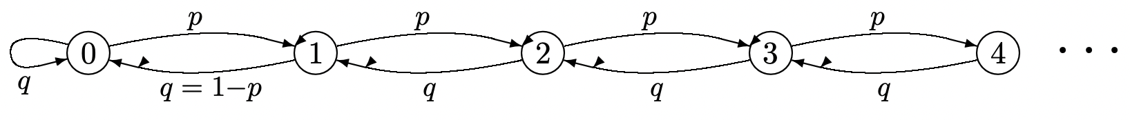
Consider the familiar Bernoulli process \(\left\{S_{n}=X_{1}+\cdots X_{n} ; n \geq 1\right\}\) where \(\left\{X_{n} ; n \geq 1\right\}\) is an IID binary sequence with \(\mathrm{p}_{X}(1)=p\) and \(\mathrm{p}_{X}(-1)=(1-p)=q\). The sequence \(\left\{S_{n} ; n \geq 1\right\}\) is a sequence of integer random variables (rv’s ) where \(S_{n}=S_{n-1}+1\) with probability p and \(S_{n}=S_{n-1}-1\) with probability \(q\). This sequence can be modeled by the Markov chain in Figure 5.1.

Figure 5.1: A Markov chain with a countable state space modeling a Bernoulli process. If \(p>1 / 2\), then as time \(n\) increases, the state \(X_{n}\) becomes large with high probability, i.e., \(\lim _{n \rightarrow \infty} \operatorname{Pr}\left\{X_{n} \geq j\right\}=1\) for each integer \(j\). Similarly, for \(p<1 / 2\), the state becomes highly negative.

Using the notation of Markov chains, \(P_{0 j}^{n}\) is the probability of being in state \(j\) at the end of the \(n\)th transition, conditional on starting in state 0. The final state \(j\) is the number of positive transitions \(k\) less the number of negative transitions \(n-k\), i.e., \(j=2 k-n\). Thus, using the binomial formula,

\[P_{0 j}^{n}=\left(\begin{array}{l}
n \\
k
\end{array}\right) p^{k} q^{n-k} \quad \text { where } k=\frac{j+n}{2} ; \quad j+n \text { even. }\label{5.1} \]

All states in this Markov chain communicate with all other states, and are thus in the same class. The formula makes it clear that this class, i.e., the entire set of states in the Markov chain, is periodic with period 2. For \(n\) even, the state is even and for \(n\) odd, the state is odd.

What is more important than the periodicity, however, is what happens to the state probabilities for large \(n\). As we saw in \ref{1.88} while proving the central limit theorem for the binomial case,

\[P_{0 j}^{n} \sim \frac{1}{\sqrt{2 \pi n p q}} \exp \left[\frac{-(k-n p)^{2}}{2 p q n}\right]^\} \quad \text { where } k=\frac{j+n}{2} ; \quad j+n \text { even.} \label{5.2} \]

In other words, \(P_{0 j}^{n}\), as a function of \(j\), looks like a quantized form of the Gaussian density for large \(n\). The significant terms of that distribution are close to \(k=n p\), i.e., to \(j=n(2 p-1)\). For \(p>1 / 2\), the state increases with increasing \(n\). Its distribution is centered at \(n(2 p-1)\), but the distribution is also spreading out as \(\sqrt{n}\). For \(p<1 / 2\), the state similarly decreases and spreads out. The most interesting case is \(p=1 / 2\), where the distribution remains centered at 0, but due to the spreading, the PMF approaches 0 as \(1 / \sqrt{n}\) for all \(j\).

For this example, then, the probability of each state approaches zero as \(n \rightarrow \infty\), and this holds for all choices of \(p\), \(0<p<1\). If we attempt to define a steady-state probability as 0 for each state, then these probabilities do not sum to 1, so they cannot be viewed as a steady-state distribution. Thus, for countable-state Markov chains, the notions of recurrence and steady-state probabilities will have to be modified from that with finitestate Markov chains. The same type of situation occurs whenever \(\left\{S_{n} ; n \geq 1\right\}\) is a sequence of sums of arbitrary IID integer-valued rv’s.

Most countable-state Markov chains that are useful in applications are quite di↵erent from Example 5.1.1, and instead are quite similar to finite-state Markov chains. The following example bears a close resemblance to Example 5.1.1, but at the same time is a countablestate Markov chain that will keep reappearing in a large number of contexts. It is a special case of a birth-death process, which we study in Section 5.2.

Example 5.1.2

Figure 5.2 is similar to Figure 5.1 except that the negative states have been eliminated. A sequence of IID binary rv’s \(\left\{X_{n} ; n \geq 1\right\}\), with \(\mathrm{p}_{X}(1)=p\) and \(\mathrm{p}_{X}(-1)=q=1-p\), controls the state transitions. Now, however, \(S_{n}=\max \left(0, S_{n-1}+X_{n}\right.\), so that \(S_{n}\) is a nonnegative rv. All states again communicate, and because of the self transition at state 0, the chain is aperiodic.

For \(p>1 / 2\), transitions to the right occur with higher frequency than transitions to the left. Thus, reasoning heuristically, we expect the state \(S_{n}\) at time \(n\) to drift to the right with increasing \(n\). Given \(S_{0}=0\), the probability \(P_{0 j}^{n}\) of being in state \(j\) at time \(n\), should then tend to zero for any fixed \(j\) with increasing \(n\). As in Example 5.1.1, we see that a steady state does not exist. In more poetic terms, the state wanders off into the wild blue yonder.

Figure 5.2: A Markov chain with a countable state space. If \(p>1 / 2\), then as time \(n\) increases, the state \(X_{n}\) becomes large with high probability, i.e., \(\lim _{n \rightarrow \infty} \operatorname{Pr}\left\{X_{n} \geq j\right\}=1\) for each integer \(j\).

One way to understand this chain better is to look at what happens if the chain is truncated. The truncation of Figure 5.2 to \(k\) states is analyzed in Exercise 3.9. The solution there defines \(\rho=p / q\) and shows that if \(\rho \neq 1\), then \(\pi_{i}=(1-\rho) \rho^{i} /\left(1-\rho^{k}\right)\) for each \(i\), \(0 \leq i<k\). For \(\rho=1\), \(\pi_{i}=1 / k\) for each \(i\). For \(\rho<1\), the limiting behavior as \(k \rightarrow \infty\) is \(\pi_{i}=(1-\rho) \rho^{i}\). Thus for \(\rho<1(p<1 / 2)\), the steady state probabilities for the truncated Markov chain approaches a limit which we later interpret as the steady state probabilities for the untruncated chain. For \(\rho>1(p>1 / 2)\), on the other hand, the steady-state probabilities for the truncated case are geometrically decreasing from the right, and the states with significant probability keep moving to the right as \(k\) increases. Although the probability of each fixed state \(j\) approaches 0 as \(k\) increases, the truncated chain never resembles the untruncated chain.

Perhaps the most interesting case is that where \(p=1 / 2\). The \(n\)th order transition probabilities, \(P_{0 j}^{n}\) can be calculated exactly for this case (see Exercise 5.3) and are very similar to those of Example 5.1.1. In particular,

\[P_{0 j}^{n}= \begin{cases}\left(\begin{array}{c}
n \\
(j+n) / 2
\end{array}\right) 2^{-n} & \text { for } j \geq 0,(j+n) \text { even } \\
\} \\
\left(\underset{(j+n+1) / 2}{n}\right) 2^{-n} & \text { for } j \geq 0,(j+n) \text { odd }\end{cases} \label{5.3} \]

\[\sim \sqrt{\frac{\}2}{\pi n}} \exp \left[\frac{-j^{2}}{2 n}\right] \quad \text { for } j \geq 0\label{5.4} \]

We see that \(P_{0 j}^{n}\) for large \(n\) is approximated by the positive side of a quantized Gaussian distribution. It looks like the positive side of the PMF of \ref{5.1} except that it is no longer periodic. For large \(n\), \(P_{0 j}^{n}\) is concentrated in a region of width \(\sqrt{n}\) around \(j = 0\), and the PMF goes to 0 as \(1 / \sqrt{n}\) for each \(j\) as \(n \rightarrow \infty\).

Fortunately, the strange behavior of Figure 5.2 when \(p \geq q\) is not typical of the Markov chains of interest for most applications. For typical countable-state Markov chains, a steady state does exist, and the steady-state probabilities of all but a finite number of states (the number depending on the chain and the application) can almost be ignored for numerical calculations.

Using renewal theory to classify and analyze Markov chains

The matrix approach used to analyze finite-state Markov chains does not generalize easily to the countable-state case. Fortunately, renewal theory is ideally suited for this purpose, especially for analyzing the long term behavior of countable-state Markov chains. We must first revise the definition of recurrent states. The definition for finite-state Markov chains does not apply here, and we will see that, under the new definition, the Markov chain in Figure 5.2 is recurrent for \(p \leq 1 / 2\) and transient for \(p>1 / 2\). For \(p=1 / 2\), the chain is called null-recurrent, as explained later.

In general, we will find that for a recurrent state \(j\), the sequence of subsequent entries to state \(j\), conditional on starting in \(j\), forms a renewal process. The renewal theorems then specify the time-average relative-frequency of state \(j\), the limiting probability of \(j\) with increasing time and a number of other relations.

We also want to understand the sequence of epochs at which one state, say \(j\), is entered, conditional on starting the chain at some other state, say \(i\). We will see that, subject to the classification of states \(i\) and \(j\), this gives rise to a delayed renewal process. In preparing to study these renewal processes and delayed renewal process, we need to understand the inter-renewal intervals. The probability mass functions (PMF’s) of these intervals are called first-passage-time probabilities in the notation of Markov chains.

Definition 5.1.1

The first-passage-time probability, \(f_{i j}(n)\), of a Markov chain is the probability, conditional on \(X_{0}=i\), that the first subsequent entry to state \(j\) occurs at discrete epoch \(n\). That is, \(f_{i j}(1)=P_{i j}\) and for \(n \geq 2\),

\[f_{i j}(n)=\operatorname{Pr}\left\{X_{n}=j, X_{n-1} \neq j, X_{n-2} \neq j, \ldots, X_{1} \neq j \mid X_{0}=i\right\}\label{5.5} \]

The distinction between \(f_{i j}(n)\) and \(P_{i j}^{n}=\operatorname{Pr}\left\{X_{n}=j \mid X_{0}=i\right\}\) is that \(f_{i j}(n)\) is the probability that the first entry to \(j\) (after time 0) occurs at time \(n\), whereas \(P_{i j}^{n}\) is the probability that any entry to \(j\) occurs at time \(n\), both conditional on starting in state \(i\) at time 0. The definition in \ref{5.5} also applies for \(j = i\); \(f_{i i}(n)\) is thus the probability, given \(X_{0}=i\), that the first occurrence of state \(i\) after time 0 occurs at time \(n\). Since the transition probabilities are independent of time, \(f_{k j}(n-1)\) is also the probability, given \(X_{1}=k\), that the first subsequent occurrence of state \(j\) occurs at time \(n\). Thus we can calculate \(f_{i j}(n)\) from the iterative relations

\[f_{i j}(n)=\sum_{k \neq j} P_{i k} f_{k j}(n-1) ; \quad n>1 ; \quad f_{i j}(1)=P_{i j}\label{5.6} \]

Note that the sum excludes \(k=j\), since \(P_{i j} f_{j j}(n-1)\) is the probability that state \(j\) occurs first at epoch 1 and next at epoch \(n\). Note also from the Chapman-Kolmogorov equation that \(P_{i j}^{n}=\sum_{k} P_{i k} P_{k j}^{n-1}\). In other words, the only di↵erence between the iterative expressions to calculate \(f_{i j}(n)\) and \(P_{i j}^{n}\) is the exclusion of \(k=j\) in the expression for \(fij (n)\).

With this iterative approach, the first-passage-time probabilities \(fij(n)\) for a given \(n\) must be calculated for all \(i\) before proceeding to calculate them for the next larger value of \(n\). This also gives us \(fjj(n)\), although \(fjj(n)\) is not used in the iteration.

Let \(\mathrm{F}_{i j}(n)\), for \(n \geq 1\), be the probability, given \(X_{0}=i\), that state \(j\) occurs at some time between 1 and \(n\) inclusive. Thus,

\[\left.\mathrm{F}_{i j}(n)=\sum_{m=1}^{n}\right\} f_{i j}(m)\label{5.7} \]

For each \(i\), \(j\), \(Fij(n)\) is non-decreasing in n and (since it is a probability) is upper bounded by 1. Thus \(\mathrm{F}_{i j}(\infty)\) (i.e., \(\lim _{n \rightarrow \infty} \mathrm{F}_{i j}(n)\)) must exist, and is the probability, given \(X_{0}=i\), that state j will ever occur. If \(\mathrm{F}_{i j}(\infty)=1\), then, given \(X_{0}=i\), it is certain (with probability 1) that the chain will eventually enter state \(j\). In this case, we can define a random variable (rv) \(T_{i j}\), conditional on \(X_{0}=i\), as the first-passage time from \(i\) to \(j\). Then \(f_{i j}(n)\) is the PMF of \(T_{i j}\) and \(\mathrm{F}_{i j}(n)\) is the distribution function of \(T_{i j}\). If \(\mathrm{F}_{i j}(\infty)<1\), then \(T_{i j}\) is a defective rv, since, with some non-zero probability, there is no first-passage to \(j\). Defective rv’s are not considered to be rv’s (in the theorems here or elsewhere), but they do have many of the properties of rv’s.

The first-passage time \(T_{j j}\) from a state \(j\) back to itself is of particular importance. It has the PMF \(f_{j j}(n)\) and the distribution function \(\mathrm{F}_{j j}(n)\). It is a rv (as opposed to a defective rv) if \(F_{j j}(\infty)=1\), i.e., if the state eventually returns to state \(j\) with probability 1 given that it starts in state \(j\). This leads to the definition of recurrence.

Definition 5.1.2

A state j in a countable-state Markov chain is recurrent if \(\mathrm{F}_{j j}(\infty)=1\). It is transient if \(\mathrm{F}_{j j}(\infty)<1\).

Thus each state \(j\) in a countable-state Markov chain is either recurrent or transient, and is recurrent if and only if an eventual return to \(j\) (conditional on \(X_{0}=j\)) occurs with probability 1. Equivalently, \(j\) is recurrent if and only if \(T_{j j}\), the time of first return to \(j\), is a rv. Note that for the special case of finite-state Markov chains, this definition is consistent with the one in Chapter 3. For a countably-infinite state space, however, the earlier definition is not adequate. An example is provided by the case \(p>1 / 2\) in Figure 5.2. Here \(i\) and \(j\) communicate for all states \(i\) and \(j\), but it is intuitively obvious (and shown in Exercise 5.2, and further explained in Section 5.2) that each state is transient.

If the initial state \(X_{0}\) of a Markov chain is a recurrent state \(j\), then \(T_{j j}\) is the integer time of the first recurrence of state \(j\). At that recurrence, the Markov chain is in the same state \(j\) as it started in, and the discrete interval from \(T_{j j}\) to the next occurrence of state \(j\), say \(T_{j j, 2}\) has the same distribution as \(T_{j j}\) and is clearly independent of \(T_{j j}\). Similarly, the sequence of successive recurrence intervals, \(T_{j j}, T_{j j, 2}, T_{j j, 3}, \ldots\) is a sequence of IID rv’s. This sequence of recurrence intervals¹ is then the sequence of inter-renewal intervals of a renewal process, where each renewal interval has the distribution of \(T_{j j}\). These inter-renewal intervals have the PMF \(f_{j j}(n)\) and the distribution function \(\mathrm{F}_{j j}(n)\).

Since results about Markov chains depend very heavily on whether states are recurrent or transient, we will look carefully at the probabilities \(\mathrm{F}_{i j}(n)\). Substituting \ref{5.6} into (5.7), we obtain

\[\left.\mathrm{F}_{i j}(n)=P_{i j}+\sum_{k \neq j}\right\} P_{i k} \mathrm{~F}_{k j}(n-1) ; \quad n>1 ; \quad \mathrm{F}_{i j}(1)=P_{i j}\label{5.8} \]

To understand the expression \(P_{i j}+\sum_{k \neq j} P_{i k} \mathrm{~F}_{k j}(n-1)\), note that the first term, \(P_{i j}\), is \(f_{i j}\) \ref{1} and the second term, \(\sum_{k \neq j} P_{i k} \mathrm{~F}_{k j}(n-1)\), is equal to \(\sum_{\ell=2}^{n} f_{i j}(\ell)\).

We have seen that \(\mathrm{F}_{i j}(n)\) is non-decreasing in n and upper bounded by 1, so the limit \(\mathrm{F}_{i j}(\infty)\) must exist. Similarly, \(\sum_{k \neq j} P_{i k} \mathrm{~F}_{k j}(n-1)\) is non-decreasing in \(n\) and upper bounded by 1, so it also has a limit, equal to \(\sum_{k \neq j} P_{i k} \mathrm{~F}_{k j}(\infty)\). Thus

\[\left.\mathrm{F}_{i j}(\infty)=P_{i j}+\sum_{k \neq j}\right\} P_{i k} \mathrm{~F}_{k j}(\infty)\label{5.9} \]

For any given \(j\), \ref{5.9} can be viewed as a set of linear equations in the variables \(\mathrm{F}_{i j}(\infty)\) for each state \(i\). There is not always a unique solution to this set of equations. In fact, the set of equations

\[x_{i j}=P_{i j}+\sum_{k \neq j} P_{i k} x_{k j} ; \quad \text { all states } i\label{5.10} \]

always has a solution in which \(x_{i j}=1\) for all \(i\). If state \(j\) is transient, however, there is another solution in which \(x_{i j}\) is the true value of \(\mathrm{F}_{i j}(\infty)\) and \(\mathrm{F}_{j j}(\infty)<1\). Exercise 5.1 shows that if \ref{5.10} is satisfied by a set of nonnegative numbers \(\left\{x_{i j} ; 1 \leq i \leq J\right\}\), then \(\mathrm{F}_{i j}(\infty) \leq x_{i j}\) for each \(i\).

We have defined a state j to be recurrent if \(\mathrm{F}_{j j}(\infty)=1\) and have seen that if \(j\) is recurrent, then the returns to state \(j\), given \(X_{0}=j\) form a renewal process. All of the results of renewal theory can then be applied to the random sequence of integer times at which \(j\) is entered. The main results from renewal theory that we need are stated in the following lemma.

Lemma 5.1.1

Let \(\left\{N_{j j}(t) ; t \geq 0\right\}\) be the counting process for occurrences of state j up to time \(t\) in a Markov chain with \(X_{0}=j\). The following conditions are then equivalent.

1. state \(j\) is recurrent.
2. \(\lim _{t \rightarrow \infty} N_{j j}(t)=\infty\) with probability 1.
3. \(\lim _{t \rightarrow \infty} \mathrm{E}\left[N_{j j}(t)\right]=\infty\)
4. \(\lim _{t \rightarrow \infty} \sum_{1 \leq n \leq t} P_{j j}^{n}=\infty\)

Proof

First assume that \(j\) is recurrent, i.e., that \(\mathrm{F}_{j j}(\infty)=1\). This implies that the interrenewal times between occurrences of \(j\) are IID rv’s, and consequently \(\left\{N_{j j}(t) ; t \geq 1\right\}\) is a renewal counting process. Recall from Lemma 4.3.1 of Chapter 4 that, whether or not the expected inter-renewal time \(\mathrm{E}\left[T_{j j}\right]\) is finite, \(\lim _{t \rightarrow \infty} N_{j j}(t)=\infty\) with probability 1 and \(\lim _{t \rightarrow \infty} \mathrm{E}\left[N_{j j}(t)\right]=\infty\).

Next assume that state \(j\) is transient. In this case, the inter-renewal time \(T_{j j}\) is not a rv, so \(\left\{N_{j j}(t) ; t \geq 0\right\}\) is not a renewal process. An eventual return to state \(j\) occurs only with probability \(\mathrm{F}_{j j}(\infty)<1\), and, since subsequent returns are independent, the total number of returns to state \(j\) is a geometric rv with mean \(\mathrm{F}_{j j}(\infty) /\left[1-\mathrm{F}_{j j}(\infty)\right]\). Thus the total number of returns is finite with probability 1 and the expected total number of returns is finite. This establishes the first three equivalences.

Finally, note that \(P_{j j}^{n}\), the probability of a transition to state \(j\) at integer time \(n\), is equal to the expectation of a transition to \(j\) at integer time \(n\) (i.e., a single transition occurs with probability \(P_{j j}^{n}\) and 0 occurs otherwise). Since \(N_{j j}(t)\) is the sum of the number of transitions to \(j\) over times 1 to \(t\), we have

\(\left.\mathrm{E}\left[N_{j j}(t)\right]=\sum_{1 \leq n \leq t}\right\} P_{j j}^{n},\)

which establishes the final equivalence.

Our next objective is to show that all states in the same class as a recurrent state are also recurrent. Recall that two states are in the same class if they communicate, i.e., each has a path to the other. For finite-state Markov chains, the fact that either all states in the same class are recurrent or all transient was relatively obvious, but for countable-state Markov chains, the definition of recurrence has been changed and the above fact is no longer obvious.

Lemma 5.1.2

If state \(j\) is recurrent and states \(i\) and \(j\) are in the same class, i.e., \(i\) and \(j\) communicate, then state i is also recurrent.

Proof

From Lemma 5.1.1, state \(j\) satisfies \(\lim _{t \rightarrow \infty} \sum_{1 \leq n \leq t} P_{j j}^{n}=\infty\). Since \(j\) and \(i\) communicate, there are integers \(m\) and \(k\) such that \(P_{i j}^{m}>0\) and \(P_{j i}^{k}>0\). For every walk from state \(j\) to \(j\) in n steps, there is a corresponding walk from \(i\) to \(i\) in \(m+n+k\) steps, going from \(i\) to \(j\) in \(m\) steps, \(j\) to \(j\) in \(n\) steps, and \(j\) back to \(i\) in \(k\) steps. Thus

\(\begin{aligned}
P_{i i}^{m+n+k} & \geq P_{i j}^{m} P_{j j}^{n} P_{j i}^{k} \\
\left.\sum_{n=1}^{\infty}\right\} P_{i i}^{n} &\left.\left.\geq \sum_{n=1}^{\infty}\right\} P_{i i}^{m+n+k} \geq P_{i j}^{m} P_{j i}^{k} \sum_{n=1}^{\infty}\right\} P_{j j}^{n}=\infty
\end{aligned}\)

Thus, from Lemma 5.1.1, \(i\) is recurrent, completing the proof.

Since each state in a Markov chain is either recurrent or transient, and since, if one state in a class is recurrent, all states in that class are recurrent, we see that if one state in a class is transient, they all are. Thus we can refer to each class as being recurrent or transient. This result shows that Theorem 3.2.1 also applies to countable-state Markov chains. We state this theorem separately here to be specific.

Theorem 5.1.1

For a countable-state Markov chain, either all states in a class are transient or all are recurrent.

We next look at the delayed counting process \(\left\{N_{i j}(n) ; n \geq 1\right\}\). If this is a delayed renewal counting process, then we can use delayed renewal processes to study whether the effect of the initial state eventually dies out. If state \(j\) is recurrent, we know that \(\left\{N_{j j}(n) ; n \geq 1\right\}\) is a renewal counting process. In addition, in order for \(\left\{N_{i j}(n) ; n \geq 1\right\}\) to be a delayed renewal counting process, it is necessary for the first-passage time to be a rv, i.e., for \(F_{i j}(\infty)\) to be 1.

Lemma 5.1.3

Let states \(i\) and \(j\) be in the same recurrent class. Then \(F_{i j}(\infty)=1\).

Proof

Since \(i\) is recurrent, the number of visits to \(i\) by time \(t\), given \(X_{0}=i\), is a renewal counting process \(N_{i i}(t)\). There is a path from \(i\) to \(j\), say of probability \(\alpha>0\). Thus the probability that the first return to \(i\) occurs before visiting \(j\) is at most \(1-\alpha\). The probability that the second return occurs before visiting \(j\) is thus at most \((1-\alpha)^{2}\) and the probability that the \(n\)th occurs without visiting \(j\) is at most \((1-\alpha)^{n}\). Since \(i\) is visited infinitely often with probability 1 as \(n \rightarrow \infty\), the probability that \(j\) is never visited is 0. Thus \(\mathrm{F}_{i j}(\infty)=1\).

Lemma 5.1.4

Let \(\left\{N_{i j}(t) ; t \geq 0\right\}\) be the counting process for transitions into state \(j\) up to time \(t\) for a Markov chain given \(X_{0}=i \neq j\). Then if \(i\) and \(j\) are in the same recurrent class, \(\left\{N_{i j}(t) ; t \geq 0\right\}\) is a delayed renewal process.

Proof

From Lemma 5.1.3, \(T_{i j}\), the time until the first transition into \(j\), is a rv. Also \(T_{j j}\) is a rv by definition of recurrence, and subsequent intervals between occurrences of state \(j\) are IID, completing the proof.

If \(\mathrm{F}_{i j}(\infty)=1\), we have seen that the first-passage time from \(i\) to \(j\) is a rv, i.e., is finite with probability 1. In this case, the mean time \(\overline{T}_{i j}\) to first enter state \(j\) starting from state \(i\) is of interest. Since \(T_{i j}\) is a nonnegative random variable, its expectation is the integral of its complementary distribution function,

\[\overline{T}_{i j}=1+\sum_{n=1}^{\infty}\left(1-\mathrm{F}_{i j}(n)\right)\label{5.11} \]

It is possible to have \(\mathrm{F}_{i j}(\infty)=1\) but \(\overline{T}_{i j}=\infty\). As will be shown in Section 5.2, the chain in Figure 5.2 satisfies \(\mathrm{F}_{i j}(\infty)=1\) and \(\overline{T}_{i j}<\infty\) for \(p<1 / 2\) and \(\mathrm{F}_{i j}(\infty)=1\) and \(\overline{T}_{i j}=\infty\) for \(p=1 / 2\). As discussed before, \(F_{i j}(\infty)<1\) for \(p>1 / 2\). This leads us to the following definition.

Definition 5.1.3

A state \(j\) in a countable-state Markov chain is positive-recurrent if \(\mathrm{F}_{j j}(\infty)=1\) and \(\overline{T}_{j j}<\infty\). It is null-recurrent if \(\mathrm{F}_{j j}(\infty)=1\) and \(\overline{T}_{j j}=\infty\).

Each state of a Markov chain is thus classified as one of the following three types — positiverecurrent, null-recurrent, or transient. For the example of Figure 5.2, null-recurrence lies on a boundary between positive-recurrence and transience, and this is often a good way to look at null-recurrence. Part f) of Exercise 6.3 illustrates another type of situation in which null-recurrence can occur.

Assume that state \(j\) is recurrent and consider the renewal process \(\left\{N_{j j}(t) ; t \geq 0\right\}\). The limiting theorems for renewal processes can be applied directly. From the strong law for renewal processes, Theorem 4.3.1,

\[\lim _{t \rightarrow \infty} N_{j j}(t) / t=1 / \overline{T}_{j j} \quad \text { with probability } 1\label{5.12} \]

From the elementary renewal theorem, Theorem 4.6.1,

\[\lim _{t \rightarrow \infty} \mathrm{E}\left[N_{j j}(t) / t\right]=1 / \overline{T}_{j j}\label{5.13} \]

Equations \ref{5.12} and \ref{5.13} are valid whether \(j\) is positive-recurrent or null-recurrent.

Next we apply Blackwell’s theorem to \(\left\{N_{j j}(t) ; t \geq 0\right\}\). Recall that the period of a given state \(j\) in a Markov chain (whether the chain has a countable or finite number of states) is the greatest common divisor of the set of integers \(n>0\) such that \(P_{j j}^{n}>0\). If this period is \(d\), then \(\left\{N_{j j}(t) ; t \geq 0\right\}\) is arithmetic with span \(\lambda\) (i.e., renewals occur only at times that are multiples of \(\lambda\). From Blackwell’s theorem in the arithmetic form of (4.61),

\[\lim _{n \rightarrow \infty} \operatorname{Pr}\left\{X_{n \lambda}=j \mid X_{0}=j\right\}=\lambda / \overline{T}_{j j}\label{5.14} \]

If state \(j\) is aperiodic (i.e., \(\lambda=1\)), this says that \(\lim _{n \rightarrow \infty} \operatorname{Pr}\left\{X_{n}=j \mid X_{0}=j\right\}=1 / \overline{T}_{j j}\). Equations \ref{5.12} and \ref{5.13} suggest that \(1 / \overline{T}_{j j}\) has some of the properties associated with a steady-state probability of state \(j\), and \ref{5.14} strengthens this if \(j\) is aperiodic. For a Markov chain consisting of a single class of states, all positive-recurrent, we will strengthen this association further in Theorem 5.1.4 by showing that there is a unique steady-state distribution, \(\left\{\pi_{j}, j \geq 0\right\}\) such that \(\pi_{j}=1 / \overline{T}_{j j}\) for all \(j\) and such that \(\pi_{j}=\sum_{i} \pi_{i} P_{i j}\) for all \(j \geq 0\) and \(\sum_{j} \pi_{j}=1\). The following theorem starts this development by showing that (5.12-5.14) are independent of the starting state.

Theorem 5.1.2

Let \(j\) be a recurrent state in a Markov chain and let i be any state in the same class as \(j\). Given \(X_{0}=i\), let \(N_{i j}(t)\) be the number of transitions into state \(j\) by time \(t\) and let \(\overline{T}_{j j}\) be the expected recurrence time of state \(j\) (either finite or infinite). Then

\[\lim _{t \rightarrow \infty} N_{i j}(t) / t=1 / \overline{T}_{j j} \quad \text { with probability } 1\label{5.15} \]

\[\lim _{t \rightarrow \infty} \mathrm{E}\left[N_{i j}(t) / t\right]=1 / \overline{T}_{j j}\label{5.16} \]

If \(j\) is also aperiodic, then

\[\lim _{n \rightarrow \infty} \operatorname{Pr}\left\{X_{n}=j \mid X_{0}=i\right\}=1 / \overline{T}_{j j}\label{5.17} \]

Proof

Since i and j are recurrent and in the same class, Lemma 5.1.4 asserts that \(\left\{N_{i j}(t) ; t \geq 0\right\}\) is a delayed renewal process for \(j \neq i\). Thus \ref{5.15} and \ref{5.16} follow from Theorems 4.8.1 and 4.8.2 of Chapter 4. If \(j\) is aperiodic, then \(\left\{N_{i j}(t) ; t \geq 0\right\}\) is a delayed renewal process for which the inter-renewal intervals \(T_{j j}\) have span 1 and \(T_{i j}\) has an integer span. Thus, \ref{5.17} follows from Blackwell’s theorem for delayed renewal processes, Theorem 4.8.3. For \(i=j\), (5.15-5.17) follow from (5.12-5.14), completing the proof.

Theorem 5.1.3

All states in the same class of a Markov chain are of the same type — either all positive-recurrent, all null-recurrent, or all transient.

Proof

Let \(j\) be a recurrent state. From Theorem 5.1.1, all states in a class are recurrent or all are transient. Next suppose that \(j\) is positive-recurrent, so that \(1 / \overline{T}_{j j}>0\). Let \(i\) be in the same class as \(j\), and consider the renewal-reward process on \(\left\{N_{j j}(t) ; t \geq 0\right\}\) for which \(R(t)=1\) whenever the process is in state \(i\) (i.e., if \(X_{n}=i\), then \(R(t)=1\) for \(n \leq t<n+1\)). The reward is 0 whenever the process is in some state other than \(i\). Let \(\mathrm{E}\left[\mathrm{R}_{n}\right]\) be the expected reward in an inter-renewal interval; this must be positive since i is accessible from \(j\). From the strong law for renewal-reward processes, Theorem 4.4.1,

\(\lim _{t \rightarrow \infty} \frac{1}{t} \int_{0}^{\}t} R(\tau) d \tau=\frac{\mathrm{E}\left[\mathrm{R}_{n}\right]}{\overline{T}_{j j}} \quad \text { with probability } 1\).

The term on the left is the time-average number of transitions into state \(i\), given \(X_{0}=j\), and this is \(1 / \overline{T}_{i i}\) from (5.15). Since \(\mathrm{E}\left[\mathrm{R}_{n}\right]>0\) and \(\overline{T}_{j j}<\infty\), we have \(1 / \overline{T}_{i i}>0\), so \(i\) is positive-recurrent. Thus if one state is positive-recurrent, the entire class is, completing the proof.

If all of the states in a Markov chain are in a null-recurrent class, then \(1 / \overline{T}_{j j}=0\) for each state, and one might think of \(1 / \overline{T}_{j j}=0\) as a “steady-state” probability for \(j\) in the sense that 0 is both the time-average rate of occurrence of \(j\) and the limiting probability of \(j\). However, these “probabilities” do not add up to 1, so a steady-state probability distribution does not exist. This appears rather paradoxical at first, but the example of Figure 5.2, with \(p=1 / 2\) will help to clarify the situation. As time \(n\) increases (starting in state \(i\), say), the random variable \(X_{n}\) spreads out over more and more states around \(i\), and thus is less likely to be in each individual state. For each \(j\), \(\lim _{n \rightarrow \infty} P_{i j}(n)=0\). Thus, \(\sum_{j}\left\{\lim _{n \rightarrow \infty} P_{i j}^{n}\right\}=0\). On the other hand, for every \(n\), \(\sum_{j} P_{i j}^{n}=1\). This is one of those unusual examples where a limit and a sum cannot be interchanged.

In Chapter 3, we defined the steady-state distribution of a finite-state Markov chain as a probability vector \(\pi\) that satisfies \(\boldsymbol{\pi}=\boldsymbol{\pi}[P]\). Here we define \(\left\{\pi_{i} ; i \geq 0\right\}\) in the same way, as a set of numbers that satisfy

\[\left.\pi_{j}=\sum_{i}\right\}_{\pi_{i} P_{i j}} \text { for all } j ; \quad \pi_{j} \geq 0 \quad \text { for all } j ; \quad \sum_{j} \pi_{j}=1\label{5.18} \]

Suppose that a set of numbers \(\left\{\pi_{i} ; i \geq 0\right\}\) satisfying \ref{5.18} is chosen as the initial probability distribution for a Markov chain, i.e., if \(\operatorname{Pr}\left\{X_{0}=i\right\}=\pi_{i}\) for all \(i\). Then \(\mathrm{Pr}\{X_1=j\}=\sum_{i} \pi_{i} P_{i j}=\pi_{j}\) for all \(j\), and, by induction, \(\operatorname{Pr}\left\{X_{n}=j\right\}=\pi_{j}\) for all \(j\) and all \(n \geq 0\). The fact that \(\operatorname{Pr}\left\{X_{n}=j\right\}=\pi_{j}\) for all \(j\) motivates the definition of steady-state distribution above. Theorem 5.1.2 showed that \(1 / \overline{T}_{j j}\) is a ‘steady-state’ probability for state \(j\), both in a time-average and a limiting ensemble-average sense. The following theorem brings these ideas together. An irreducible Markov chain is a Markov chain in which all pairs of states communicate. For finite-state chains, irreducibility implied a single class of recurrent states, whereas for countably infinite chains, an irreducible chain is a single class that can be transient, null-recurrent, or positive-recurrent.

Theorem 5.1.4

Assume an irreducible Markov chain with transition probabilities \(\left\{P_{i j}\right\}\). If \ref{5.18} has a solution, then the solution is unique, \(\pi_{i}=1 / \overline{T}_{i i}>0\) for all \(i \geq 0\), and the states are positive-recurrent. Also, if the states are positive-recurrent then \ref{5.18} has a solution.

Proof

Let \(\left\{\pi_{j} ; j \geq 0\right\}\) satisfy \ref{5.18} and be the initial distribution of the Markov chain, i.e., \(\operatorname{Pr}\left\{X_{0}=j\right\}=\pi_{j}, j \geq 0\). Then, as shown above, \(\operatorname{Pr}\left\{X_{n}=j\right\}=\pi_{j}\) for all \(n \geq 0, j \geq 0\). Let \(\tilde{N}_{j}(t)\) be the number of occurrences of any given state \(j\) from time 1 to \(t\). Equating \(\operatorname{Pr}\left\{X_{n}=j\right\}\) to the expectation of an occurrence of \(j\) at time \(n\), we have,

\(\left.\left.(1 / t) \mathrm{E}\left[\tilde{N}_{j}(t)\right]\right\}=(1 / t) \sum_{1 \leq n \leq t}\right\} \operatorname{Pr}\left\{X_{n}=j\right\}=\pi_{j} \quad \text { for all integers } t \geq 1\)

Conditioning this on the possible starting states i, and using the counting processes \(\left\{N_{i j}(t) ; t \geq0\right.\}\) defined earlier,

\[\pi_{j}=(1 / t) \mathrm{E}\left[\tilde{N}_{j}(t)\right]^\}=\sum_{i} \pi_{i} \mathrm{E}\left[N_{i j}(t) / t\right] \quad \text { for all integer } t \geq 1\label{5.19} \]

For any given state \(i\), let \(T_{i j}\) be the time of the first occurrence of state \(j\) given \(X_{0}=i\). Then if \(T_{i j}<\infty\), we have \(N_{i j}(t) \leq N_{i j}\left(T_{i j}+t\right)\). Thus, for all \(t \geq 1\),

\[\mathrm{E}\left[N_{i j}(t)\right] \leq \mathrm{E}\left[N_{i j}\left(T_{i j}+t\right)\right]=1+\mathrm{E}\left[N_{j j}(t)\right]\label{5.20} \]

The last step follows since the process is in state \(j\) at time \(T_{i j}\), and the expected number of occurrences of state \(j\) in the next \(t\) steps is \(\mathrm{E}\left[N_{j j}(t)\right]\).

Substituting \ref{5.20} in \ref{5.19} for each \(i\), \(\left.\pi_{j} \leq 1 / t+\mathrm{E}\left[N_{j j}(t) / t\right)\right]\). Taking the limit as \(t \rightarrow \infty\) and using (5.16), \(\pi_{j} \leq \lim _{t \rightarrow \infty} \mathrm{E}\left[N_{j j}(t) / t\right]\). Since \(\sum_{i} \pi_{i}=1\), there is at least one value of \(j\) for which \(\pi_{j}>0\), and for this \(j\), \(\lim _{t \rightarrow \infty} \mathrm{E}\left[N_{j j}(t) / t\right]>0\), and consequently \(\lim _{t \rightarrow \infty} \mathrm{E}\left[N_{j j}(t)\right]=\infty\). Thus, from Lemma 5.1.1, state \(j\) is recurrent, and from Theorem 5.1.2, \(j\) is positive-recurrent. From Theorem 5.1.3, all states are then positive-recurrent. For any \(j\) and any integer \(M\), \ref{5.19} implies that

\[\left.\pi_{j} \geq \sum_{i \leq M}\right\} \pi_{i} \mathrm{E}\left[N_{i j}(t) / t\right] \quad \text { for all } t\label{5.21} \]

From Theorem 5.1.2, \(\lim _{t \rightarrow \infty} \mathrm{E}\left[N_{i j}(t) / t\right]=1 / \overline{T}_{j j}\) for all \(i\). Substituting this into (5.21), we get \(\pi_{j} \geq 1 / \overline{T}_{j j} \sum_{i \leq M} \pi_{i}\). Since \(M\) is arbitrary, \(\pi_{j} \geq 1 / \overline{T}_{j j}\). Since we already showed that \(\pi_{j} \leq \lim _{t \rightarrow \infty} \mathrm{E}\left[N_{j j}(t) / t\right]=1 / \overline{T}_{j j}\), we have \(\pi_{j}=1 / \overline{T}_{j j}\) for all \(j\). This shows both that \(\pi_{j}>0\) for all \(j\) and that the solution to \ref{5.18} is unique. Exercise 5.5 completes the proof by showing that if the states are positive-recurrent, then choosing \(\pi_{j}=1 / \overline{T}_{j j}\) for all \(j\) satisfies (5.18).

In practice, it is usually easy to see whether a chain is irreducible. We shall also see by a number of examples that the steady-state distribution can often be calculated from (5.18). Theorem 5.1.4 then says that the calculated distribution is unique and that its existence guarantees that the chain is positive recurrent.

Example 5.1.3. Age of a renewal process

Consider a renewal process \(\{N(t) ; t>0\}\) in which the inter-renewal random variables \(\left\{W_{n} ; n \geq 1\right\}\) are arithmetic with span 1. We will use a Markov chain to model the age of this process (see Figure 5.3). The probability that a renewal occurs at a particular integer time depends on the past only through the integer time back to the last renewal. The state of the Markov chain during a unit interval will be taken as the age of the renewal process at the beginning of the interval. Thus, each unit of time, the age either increases by one or a renewal occurs and the age decreases to 0 (i.e., if a renewal occurs at time \(t\), the age at time \(t\) is 0).

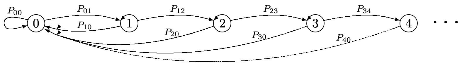Figure 5.3: A Markov chain model of the age of a renewal process.

\(\operatorname{Pr}\{W>n\}\) is the probability that an inter-renewal interval lasts for more than \(n\) time units. We assume that \(\operatorname{Pr}\{W>0\}=1\), so that each renewal interval lasts at least one time unit. The probability \(P_{n, 0}\) in the Markov chain is the probability that a renewal interval has duration \(n+1\), given that the interval exceeds \(n\). Thus, for example, \(P_{00}\) is the probability that the renewal interval is equal to 1. \(P_{n, n+1}\) is \(1-P_{n, 0}\), which is \(\operatorname{Pr}\{W>n+1\} / \operatorname{Pr}\{W>n\}\). We can then solve for the steady state probabilities in the chain: for \(n>0\),

\(\pi_{n}=\pi_{n-1} P_{n-1, n}=\pi_{n-2} P_{n-2, n-1} P_{n-1, n}=\pi_{0} P_{0,1} P_{1,2} \ldots P_{n-1, n}\).

The first equality above results from the fact that state \(n\), for \(n>0\) can be entered only from state \(n-1\). The subsequent equalities come from substituting in the same expression for \(\pi_{n-1}\), then \(p_{n-2}\), and so forth.

\[\pi_{n}=\pi_{0} \frac{\operatorname{Pr}\{W>1\} \operatorname{Pr}\{W>2\}}{\operatorname{Pr}\{W>0\} \operatorname{Pr}\{W>1\}} \cdots \frac{\operatorname{Pr}\{W>n\}}{\operatorname{Pr}\{W>n-1\}}=\pi_{0} \operatorname{Pr}\{W>n\}\label{5.22} \]

We have cancelled out all the cross terms above and used the fact that \(\operatorname{Pr}\{W>0\}=1\). Another way to see that \(\pi_{n}=\pi_{0} \operatorname{Pr}\{W>n\}\) is to observe that state 0 occurs exactly once in each inter-renewal interval; state \(n\) occurs exactly once in those inter-renewal intervals of duration \(n\) or more.

Since the steady-state probabilities must sum to 1, \ref{5.22} can be solved for \(\pi_{0}\) as

\[\pi_{0}=\frac{1}{\sum_{n=0}^{\infty} \operatorname{Pr}\{W>n\}}=\frac{1}{\mathrm{E}[W]}\label{5.23} \]

The second equality follows by expressing E [W] as the integral of the complementary distribution function of W. Combining this with (5.22), the steady-state probabilities for \(n \geq 0\) are

\[\pi_{n}=\frac{\operatorname{Pr}\{W>n\}}{\mathrm{E}[W]}\label{5.24} \]

In terms of the renewal process, \(\pi_{n}\) is the probability that, at some large integer time, the age of the process will be \(n\). Note that if the age of the process at an integer time is \(n\), then the age increases toward \(n+1\) at the next integer time, at which point it either drops to 0 or continues to rise. Thus \(\pi_{n}\) can be interpreted as the fraction of time that the age of the process is between \(n\) and \(n+1\). Recall from \ref{4.28} (and the fact that residual life and age are equally distributed) that the distribution function of the time-average age is given by \(\mathrm{F}_{Z}(n)=\int_{0}^{n} \operatorname{Pr}\{W>w\} d w / \mathrm{E}[W]\). Thus, the probability that the age is between \(n\) and \(n+1\) is \(\mathrm{F}_{Z}(n+1)-\mathrm{F}_{Z}(n)\). Since W is an integer random variable, this is \(\operatorname{Pr}\{W>n\} / \mathrm{E}[W]\) in agreement with our result here.

The analysis here gives a new, and intuitively satisfying, explanation of why the age of a renewal process is so di↵erent from the inter-renewal time. The Markov chain shows the ever increasing loops that give rise to large expected age when the inter-renewal time is heavy tailed (i.e., has a distribution function that goes to 0 slowly with increasing time). These loops can be associated with the isosceles triangles of Figure 4.7. The advantage here is that we can associate the states with steady-state probabilities if the chain is recurrent. Even when the Markov chain is null-recurrent (i.e., the associated renewal process has infinite expected age), it seems easier to visualize the phenomenon of infinite expected age.

---

¹Note that in Chapter 4 the inter-renewal intervals were denoted \(X_{1}, X_{2}, \ldots\), whereas here \(X_{0}, X_{1}, \ldots\), is the sequence of states in the Markov chain and \(T_{j j}, T_{j j, 2}, \ldots\), is the sequence of inter-renewal intervals.