5.2: Birth-Death Markov chains

A birth-death Markov chain is a Markov chain in which the state space is the set of nonnegative integers; for all \(i \geq 0\), the transition probabilities satisfy \(P_{i, i+1}>0\) and \(P_{i+1, i}>0\), and for all \(|i-j|>1, P_{i j}=0\) (see Figure 5.4). A transition from state \(i\) to \(i+1\) is regarded as a birth and one from \(i+1\) to \(i\) as a death. Thus the restriction on the transition probabilities means that only one birth or death can occur in one unit of time. Many applications of birth-death processes arise in queueing theory, where the state is the number of customers, births are customer arrivals, and deaths are customer departures. The restriction to only one arrival or departure at a time seems rather peculiar, but usually such a chain is a finely sampled approximation to a continuous-time process, and the time increments are then small enough that multiple arrivals or departures in a time increment are unlikely and can be ignored in the limit.

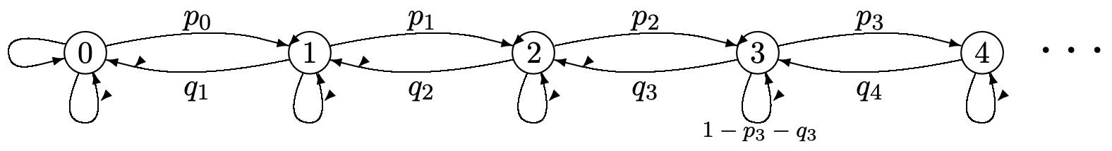Figure 5.4: Birth-death Markov chain.

We denote \(P_{i, i+1}\) by \(p_{i}\) and \(P_{i, i-1}\) by \(q_{i}\). Thus \(P_{i i}=1-p_{i}-q_{i}\). There is an easy way to find the steady-state probabilities of these birth-death chains. In any sample function of the process, note that the number of transitions from state \(i\) to \(i + 1\) differs by at most 1 from the number of transitions from \(i + 1\) to \(i\). If the process starts to the left of \(i\) and ends to the right, then one more \(i \rightarrow i+1\) transition occurs than \(i+1 \rightarrow i\), etc. Thus if we visualize a renewal-reward process with renewals on occurrences of state \(i\) and unit reward on transitions from state \(i\) to \(i+1\), the limiting time-average number of transitions per unit time is \(\pi_{i} p_{i}\). Similarly, the limiting time-average number of transitions per unit time from \(i+1\) to \(i\) is \(\pi_{i+1} q_{i+1}\). Since these two must be equal in the limit,

\[\pi_{i} p_{i}=\pi_{i+1} q_{i+1} \quad \text { for } i \geq 0\label{5.25} \]

The intuition in \ref{5.25} is simply that the rate at which downward transitions occur from \(i + 1\) to \(i\) must equal the rate of upward transitions. Since this result is very important, both here and in our later study of continuous-time birth-death processes, we show that \ref{5.25} also results from using the steady-state equations in (5.18):

\[\pi_{i}=p_{i-1} \pi_{i-1}+\left(1-p_{i}-q_{i}\right) \pi_{i}+q_{i+1} \pi_{i+1} ; \quad i>0\label{5.26} \]

\[\pi_{0}=\left(1-p_{0}\right) \pi_{0}+q_{1} \pi_{1}\label{5.27} \]

From (5.27), \(p_{0} \pi_{0}=q_{1} \pi_{1}\). To see that \ref{5.25} is satisfied for \(i>0\), we use induction on \(i\), with \(i=0\) as the base. Thus assume, for a given \(i\), that \(p_{i-1} \pi_{i-1}=q_{i} \pi_{i}\). Substituting this in (5.26), we get \(p_{i} \pi_{i}=q_{i+1} \pi_{i+1}\), thus completing the inductive proof.

It is convenient to define \(\rho_{i}\) as \(p_{i} / q_{i+1}\). Then we have \(\pi_{i+1}=\rho_{i} \pi_{i}\), and iterating this,

\[\pi_{i}=\pi_{0} \prod_{j=0}^{i-1} \rho_{j} ; \quad \pi_{0}=\frac{1}{1+\sum_{i=1}^{\infty} \prod_{j=0}^{i-1} \rho_{j}}\label{5.28} \]

If \(\sum_{i \geq 1} \prod_{0 \leq j<i} \rho_{j}<\infty\), then \(\pi_{0}\) is positive and all the states are positive-recurrent. If this sum of products is infinite, then no state is positive-recurrent. If \(\rho_{j}\) is bounded below 1, say \(\rho_{j} \leq 1-\epsilon\) for some fixed \(e>0\) and all suciently large \(j\), then this sum of products will converge and the states will be positive-recurrent.

For the simple birth-death process of Figure 5.2, if we define \(\rho=q / p\), then \(\rho_{j}=\rho\) for all \(j\). For \(\rho<1\), \ref{5.28} simplifies to \(\pi_{i}=\pi_{o} \rho^{i}\) for all \(i \geq 0\), \(\pi_{0}=1-\rho\), and thus \(\pi_{i}=(1-\rho) \rho^{i}\) for \(i \geq 0\). Exercise 5.2 shows how to find \(F_{i j}(\infty)\) for all \(i\), \(j\) in the case where \(\rho \geq 1\). We have seen that the simple birth-death chain of Figure 5.2 is transient if \(\rho>1\). This is not necessarily so in the case where self-transitions exist, but the chain is still either transient or null-recurrent. An example of this will arise in Exercise 6.3.