5.4: The M/M/1 sample-time Markov chain

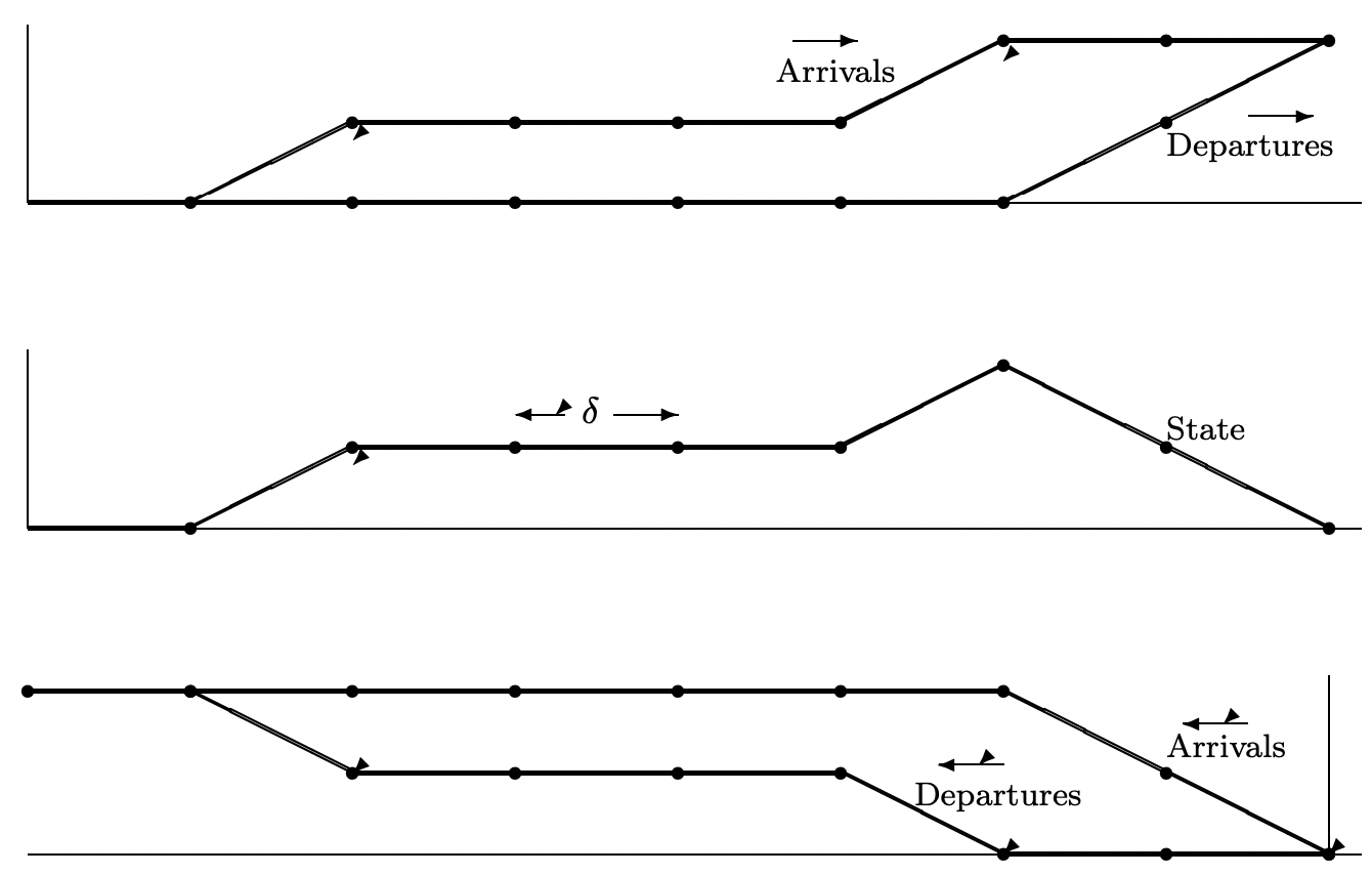
The M/M/1 Markov chain is a sampled-time model of the M/M/1 queueing system. Recall that the M/M/1 queue has Poisson arrivals at some rate and IID exponentially distributed service times at some rate \(\mu\). We assume throughout this section that \(\lambda<\mu\) (this is required to make the states positive-recurrent). For some given small increment of time \(\delta\), we visualize observing the state of the system at the sample times \(n \delta\). As indicated in Figure 5.5, the probability of an arrival in the interval from \((n-1) \delta\) to \(n \delta\) is modeled as \(\lambda \delta\), independent of the state of the chain at time \((n-1) \delta\) and thus independent of all prior arrivals and departures. Thus the arrival process, viewed as arrivals in subsequent intervals of duration \(\delta\), is Bernoulli, thus approximating the Poisson arrivals. This is a sampled-time approximation to the Poisson arrival process of rate \(\lambda\) for a continuous-time M/M/1 queue.

Figure 5.5: Sampled-time approximation to M/M/1 queue for time increment \(\delta\).

When the system is non-empty (i.e., the state of the chain is one or more), the probability of a departure in the interval \((n-1) \delta\) to \(n \delta\) is \(\mu \delta\), thus modelling the exponential service times. When the system is empty, of course, departures cannot occur.

Note that in our sampled-time model, there can be at most one arrival or departure in an interval \((n-1) \delta\) to \(n \delta\). As in the Poisson process, the probability of more than one arrival, more than one departure, or both an arrival and a departure in an increment \(\delta\) is of order \(\delta^{2}\) for the actual continuous-time M/M/1 system being modeled. Thus, for \(\delta\) very small, we expect the sampled-time model to be relatively good. At any rate, we can now analyze the model with no further approximations.

Since this chain is a birth-death chain, we can use \ref{5.28} to determine the steady-state probabilities; they are

\(\pi_{i}=\pi_{0} \rho^{i} ; \rho=\lambda / \mu<1\)

Setting the sum of the \(\pi_{i}\) to 1, we find that \(\pi_{0}=1-\rho\), so

\[\pi_{i}=(1-\rho) \rho^{i} ; \quad \text { all } i \geq 0\label{5.40} \]

Thus the steady-state probabilities exist and the chain is a birth-death chain, so from Theorem 5.3.1, it is reversible. We now exploit the consequences of reversibility to find some rather surprising results about the M/M/1 chain in steady state. Figure 5.6 illustrates a sample path of arrivals and departures for the chain. To avoid the confusion associated with the backward chain evolving backward in time, we refer to the original chain as the chain moving to the right and to the backward chain as the chain moving to the left.

There are two types of correspondence between the right-moving and the left-moving chain:

1. The left-moving chain has the same Markov chain description as the right-moving chain, and thus can be viewed as an M/M/1 chain in its own right. We still label the sampled-time intervals from left to right, however, so that the left-moving chain makes transitions from \(X_{n+1}\) to \(X_{n}\) to \(X_{n-1}\). Thus, for example, if \(X_{n}=i\) and \(X_{n-1}=i+1\), the left-moving chain has an arrival in the interval from \(n \delta\) to \((n-1) \delta\).
2. Each sample function \(\ldots x_{n-1}, x_{n}, x_{n+1} \ldots\) of the right-moving chain corresponds to the same sample function \(\ldots x_{n+1}, x_{n}, x_{n-1} \ldots\) of the left-moving chain, where \(X_{n-1}=x_{n-1}\) is to the left of \(X_{n}=x_{n}\) for both chains. With this correspondence, an arrival to the right-moving chain in the interval \((n-1) \delta\) to \(n \delta\) is a departure from the leftmoving chain in the interval \(n \delta\) to \((n-1) \delta\), and a departure from the right-moving chain is an arrival to the left-moving chain. Using this correspondence, each event in the left-moving chain corresponds to some event in the right-moving chain.

In each of the properties of the M/M/1 chain to be derived below, a property of the leftmoving chain is developed through correspondence 1 above, and then that property is translated into a property of the right-moving chain by correspondence 2.

Property 1: Since the arrival process of the right-moving chain is Bernoulli, the arrival process of the left-moving chain is also Bernoulli (by correspondence 1). Looking at a sample function \(x_{n+1}, x_{n}, x_{n-1}\) of the left-moving chain (i.e., using correspondence 2), an arrival in the interval \(n \delta\) to \((n-1) \delta\) of the left-moving chain is a departure in the interval \((n-1) \delta\) to \(n \delta\) of the right-moving chain. Since the arrivals in successive increments of the left-moving chain are independent and have probability \(\lambda \delta\) in each increment \(\delta\), we conclude that departures in the right-moving chain are similarly Bernoulli.

The fact that the departure process is Bernoulli with departure probability \(\lambda \delta\) in each increment is surprising. Note that the probability of a departure in the interval \((n \delta-\delta, n \delta]\) is \(\mu \delta\) conditional on \(X_{n-1} \geq 1\) and is 0 conditional on \(X_{n-1}=0\). Since \(\operatorname{Pr}\left\{X_{n-1} \geq 1\right\}= 1-\operatorname{Pr}\{X_{n-1}=0\}=\rho\), we see that the unconditional probability of a departure in the interval \((n \delta-\delta, n \delta]\) is \(\rho \mu \delta=\lambda \delta\) as asserted above. The fact that successive departures are independent is much harder to derive without using reversibility (see exercise 5.13).

Property 2: In the original (right-moving) chain, arrivals in the time increments after \(n \delta\) are independent of \(X_{n}\). Thus, for the left-moving chain, arrivals in time increments to the left of \(n \delta\) are independent of the state of the chain at \(n \delta\). From the correspondence between sample paths, however, a left chain arrival is a right chain departure, so that for the right-moving chain, departures in the time increments prior to \(n \delta\) are independent of \(X_{n}\), which is equivalent to saying that the state \(X_{n}\) is independent of the prior departures.

Figure 5.6: Sample function of M/M/1 chain over a busy period and corresponding arrivals and departures for right and left-moving chains. Arrivals and departures are viewed as occurring between the sample times, and an arrival in the left-moving chain between time \(n \delta\) and \((n+1) \delta\) corresponds to a departure in the right-moving chain between \((n+1) \delta\) and \(n \delta\).

This means that if one observes the departures prior to time \(n \delta\), one obtains no information about the state of the chain at \(n \delta\). This is again a surprising result. To make it seem more plausible, note that an unusually large number of departures in an interval from \((n-m) \delta\) to \(n \delta\) indicates that a large number of customers were probably in the system at time \((n-m) \delta\), but it doesn’t appear to say much (and in fact it says exactly nothing) about the number remaining at \(n \delta\).

The following theorem summarizes these results.

Theorem 5.4.1 (Burke's theorem for sampled-time).

Given an M/M/1 Markov chain in steady state with \(\lambda<\mu\),

1. the departure process is Bernoulli,
2. the state \(X_{n}\) at any time \(n \delta\) is independent of departures prior to \(n \delta\).

The proof of Burke’s theorem above did not use the fact that the departure probability is the same for all states except state 0. Thus these results remain valid for any birth-death chain with Bernoulli arrivals that are independent of the current state (i.e., for which \(P_{i, i+1}=\lambda \delta\) for all \(i \geq 0\)). One important example of such a chain is the sampled time approximation to an M/M/m queue. Here there are m servers, and the probability of departure from state \(i\) in an increment \(\delta\) is \(\mu i \delta\) for \(i \leq m\) and \(\mu m \delta\) for \(i>m\). For the states to be recurrent, and thus for a steady state to exist, \(\lambda\) must be less than \(\mu m\). Subject to this restriction, properties a) and b) above are valid for sampled-time M/M/m queues.