5.5: Branching Processes

Branching processes provide a simple model for studying the population of various types of individuals from one generation to the next. The individuals could be photons in a photomultiplier, particles in a cloud chamber, micro-organisms, insects, or branches in a data structure.

Let \(X_{n}\) be the number of individuals in generation \(n\) of some population. Each of these \(X_{n}\) individuals, independently of each other, produces a random number of offspring, and these o↵spring collectively make up generation \(n+1\). More precisely, a branching process is a Markov chain in which the state \(X_{n}\) at time \(n\) models the number of individuals in generation \(n\). Denote the individuals of generation \(n\) as \(\left\{1,2, \ldots, X_{n}\right\}\) and let \(Y_{k, n}\) be the number of o↵spring of individual \(k\). The random variables \(Y_{k, n}\) are defined to be IID over \(k\) and \(n\), with a \(\operatorname{PMF} p_{j}=\operatorname{Pr}\left\{Y_{k, n}=j\right\}\). The state at time \(n+1\), namely the number of individuals in generation \(n+1\), is

\[X_{n+1}=\sum_{k=1}^{X_{n}} Y_{k, n}\label{5.41} \]

Assume a given distribution (perhaps deterministic) for the initial state \(X_{0}\). The transition probability, \(P_{i j}=\operatorname{Pr}\left\{X_{n+1}=j \mid X_{n}=i\right\}\), is just the probability that \(Y_{1, n}+Y_{2, n}+\cdots+Y_{i, n}=j\). The zero state (i e., the state in which there are no individuals) is a trapping state (i.e., \(P_{00}=1\)) since no future o↵spring can arise in this case.

One of the most important issues about a branching process is the probability that the population dies out eventually. Naturally, if \(p_{0}\) (the probability that an individual has no offspring) is zero, then each generation must be at least as large as the generation before, and the population cannot die out unless \(X_{0}=0\). We assume in what follows that \(p_{0}>0\) and \(X_{0}>0\). Recall that \(\mathrm{F}_{i j}(n)\) was defined as the probability, given \(X_{0}=i\), that state \(j\) is entered between times 1 and \(n\). From (5.8), this satisfies the iterative relation

\[\mathrm{F}_{i j}(n)=P_{i j}+\sum_{k \neq j} P_{i k} \mathrm{~F}_{k j}(n-1), n>1 ; \quad \mathrm{F}_{i j}(1)=P_{i j}\label{5.42} \]

The probability that the process dies out by time \(n\) or before, given \(X_{0}=i\), is thus \(\mathrm{F}_{i 0}(n)\). For the \(n^{t h}\) generation to die out, starting with an initial population of \(i\) individuals, the descendants of each of those \(i\) individuals must die out. Since each individual generates descendants independently, we have \(\mathrm{F}_{i 0}(n)=\left[\mathrm{F}_{10}(n)\right]^{i}\) for all \(i\) and \(n\). Because of this relationship, it is sucient to find \(\mathrm{F}_{10}(n)\), which can be determined from (5.42). Observe that \(P_{1 k}\) is just \(p_{k}\), the probability that an individual will have \(k\) offspring. Thus, \ref{5.42} becomes

\[\left.\mathrm{F}_{10}(n)=p_{0}+\sum_{k=1}^{\infty}\right\} p_{k}\left[\mathrm{~F}_{10}(n-1)\right]^{k}=\left.\sum_{k=0}^{\infty}\right\} p_{k}\left[\mathrm{~F}_{10}(n-1)\right]^{k}\label{5.43} \]

Let \(h(z)=\sum_{k} p_{k} z^{k}\) be the \(z\) transform of the number of an individual’s offspring. Then \ref{5.43} can be written as

\[\mathrm{F}_{10}(n)=h\left(\mathrm{~F}_{10}(n-1)\right)\label{5.44} \]

This iteration starts with \(\mathrm{F}_{10}(1)=p_{0}\). Figure 5.7 shows a graphical construction for evaluating \(\mathrm{F}_{10}(n)\). Having found \(\mathrm{F}_{10}(n)\) as an ordinate on the graph for a given value of \(n\), we find the same value as an abscissa by drawing a horizontal line over to the straight line of slope 1; we then draw a vertical line back to the curve \(h(z)\) to find \(h\left(\mathrm{~F}_{10}(n)\right)=\mathrm{F}_{10}(n+1)\).

Figure 5.7: Graphical construction to find the probability that a population dies out. Here \(\mathrm{F}_{10}(n)\) is the probability that a population starting with one member at generation is the probability that a population starting with one member at generation \(F_{10}(\infty)\) is the probability that the population ever dies out.

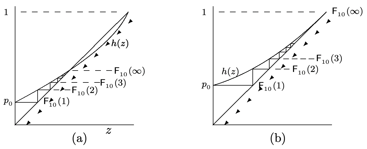
For the two subfigures shown, it can be seen that \(\mathrm{F}_{10}(\infty)\) is equal to the smallest root of the equation \(h(z)-z=0\). We next show that these two figures are representative of all possibilities. Since \(h(z)\) is a \(z\) transform, we know that \(h(1)=1\), so that \(z = 1\) is one root of \(h(z)-z=0\). Also, \(h^{\prime}(1)=\overline{Y}\), where \(\overline{Y}=\sum_{k} k p_{k}\) is the expected number of an individual’s offspring. If \(\overline{Y}>1\), as in Figure 5.7a, then \(h(z)-z\) is negative for \(z\) slightly smaller than 1. Also, for \(z=0, h(z)-z=h(0)=p_{0}>0\). Since \(h^{\prime \prime}(z) \geq 0\), there is exactly one root of \(h(z)-z=0\) for \(0<z<1\), and that root is equal to \(\mathrm{F}_{10}(\infty)\). By the same type of analysis, it can be seen that if \(\overline{Y} \leq 1\), as in Figure 5.7b, then there is no root of \(h(z)-z=0\) for \(z<1\), and \(\mathrm{F}_{10}(\infty)=1\).

As we saw earlier, \(\mathrm{F}_{i 0}(\infty)=\left[\mathrm{F}_{10}(\infty)\right]^{i}\), so that for any initial population size, there is a probability strictly between 0 and 1 that successive generations eventually die out for \(\overline{Y}>1\), and probability 1 that successive generations eventually die out for \(\overline{Y} \leq 1\). Since state 0 is accessible from all \(i\), but \(\mathrm{F}_{0 i}(\infty)=0\), it follows from Lemma 5.1.3 that all states other than state 0 are transient.

We next evaluate the expected number of individuals in a given generation. Conditional on \(X_{n-1}=i\), \ref{5.41} shows that the expected value of \(X_{n}\) is \(i \overline{Y}\). Taking the expectation over \(X_{n-1}\), we have

\[\mathrm{E}\left[X_{n}\right]=\overline{Y} \mathrm{E}\left[X_{n-1}\right]\label{5.45} \]

Iterating this equation, we get

\[\mathrm{E}\left[X_{n}\right]=\overline{Y}^{n} \mathrm{E}\left[X_{0}\right]\label{5.46} \]

Thus, if \(\overline{Y}>1\), the expected number of individuals in a generation increases exponentially with \(n\), and \(\overline{Y}\) gives the rate of growth. Physical processes do not grow exponentially forever, so branching processes are appropriate models of such physical processes only over some finite range of population. Even more important, the model here assumes that the number of offspring of a single member is independent of the total population, which is highly questionable in many areas of population growth. The advantage of an oversimplified model such as this is that it explains what would happen under these idealized conditions, thus providing insight into how the model should be changed for more realistic scenarios.

It is important to realize that, for branching processes, the mean number of individuals is not a good measure of the actual number of individuals. For \(\overline{Y}=1\) and \(X_{0}=1\), the expected number of individuals in each generation is 1, but the probability that \(X_{n}=0\) approaches 1 with increasing n; this means that as n gets large, the \(n^{t h}\) generation contains a large number of individuals with a very small probability and contains no individuals with a very large probability. For \(\overline{Y}>1\), we have just seen that there is a positive probability that the population dies out, but the expected number is growing exponentially.

A surprising result, which is derived from the theory of martingales in Chapter 7, is that if \(X_{0}=1\) and \(\overline{Y}>1\), then the sequence of random variables \(X_{n} / \overline{Y}^{n}\) has a limit with probability 1. This limit is a random variable; it has the value 0 with probability \(\mathrm{F}_{10}(\infty)\), and has larger values with some given distribution. Intuitively, for large \(n, X_{n}\) is either 0 or very large. If it is very large, it tends to grow in an orderly way, increasing by a multiple of \(\overline{Y}\) in each subsequent generation.