5.6: Round-robin and Processor Sharing

Typical queueing systems have one or more servers who each serve customers in FCFS order, serving one customer completely while other customers wait. These typical systems have larger average delay than necessary. For example, if two customers with service requirements of 10 and 1 units respectively are waiting when a single server becomes empty, then serving the first before the second results in departures at times 10 and 11, for an average delay of 10.5. Serving the customers in the opposite order results in departures at times 1 and 11, for an average delay of 6. Supermarkets have recognized this for years and have special express checkout lines for customers with small service requirements.

Giving priority to customers with small service requirements, however, has some disadvantages; first, customers with high service requirements can feel discriminated against, and second, it is not always possible to determine the service requirements of customers before they are served. The following alternative to priorities is popular both in the computer and data network industries. When a processor in a computer system has many jobs to accomplish, it often serves these jobs on a time-shared basis, spending a small increment of time on one, then the next, and so forth. In data networks, particularly high-speed networks, messages are broken into small fixed-length packets, and then the packets from different messages can be transmitted on an alternating basis between messages.

A round-robin service system is a system in which, if there are m customers in the system, say \(c_{1}, c_{2}, \ldots, c_{m}\), then \(c_{1}\) is served for an incremental interval \(\delta\), followed by \(c_{2}\) being served for an interval \(\delta\), and so forth up to \(c_{m}\). After \(c_{m}\) is served for an interval \(\delta\), the server returns and starts serving \(c_{1}\) for an interval \(\delta\) again. Thus the customers are served in a cyclic, or “round-robin” order, each getting a small increment of service on each visit from the server. When a customer’s service is completed, the customer leaves the system, \(m\) is reduced, and the server continues rotating through the now reduced cycle as before. When a new customer arrives, \(m\) is increased and the new customer must be inserted into the cycle of existing customers in a way to be discussed later.

Processor sharing is the limit of round-robin service as the increment \(\delta\) goes to zero. Thus, with processor sharing, if m customers are in the system, all are being served simultaneously, but each is being served at \(1 / m\) times the basic server rate. For the example of two customers with service requirement 1 and 10, each customer is initially served at rate 1/2, so one customer departs at time 2. At that time, the remaining customer is served at rate 1 and departs at time 11. For round-robin service with an increment of 1, the customer with unit service requirement departs at either time 1 or 2, depending on the initial order of service. With other increments of service, the results are slightly different.

We first analyze round-robin service and then go to the processor-sharing limit as \(\delta \rightarrow 0\). As the above example suggests, the results are somewhat cleaner in the limiting case, but more realistic in the round-robin case. Round robin provides a good example of the use of backward transition probabilities to find the steady-state distribution of a Markov chain. The techniques used here are quite similar to those used in the next chapter to analyze queueing networks.

Assume a Bernoulli arrival process in which the probability of an arrival in an interval \(\delta\) is \(\lambda \delta\). Assume that the \(i^{t h}\) arriving customer has a service requirement \(W_{i}\). The random variables \(W_{i}, i \geq 1\), are IID and independent of the arrival epochs. Thus, in terms of the arrival process and the service requirements, this is the same as an M/G/1 queue (see Section 4.5.5), but with M/G/1 queues, the server serves each customer completely before going on to the next customer. We shall find that the round-robin service here avoids the “slow truck effect” identified with the M/G/1 queue.

For simplicity, assume that \(W_{i}\) is arithmetic with span \(\delta\), taking on only values that are positive integer multiples of \(\delta\). Let \(f(j)=\operatorname{Pr}\left\{W_{i}=j \delta\right\}, j \geq 1\) and let \(\overline{F}(j)=\operatorname{Pr}\left\{W_{i}>j \delta\right\}\). Note that if a customer has already received j increments of service, then the probability that that customer will depart after 1 more increment is \(f(j+1) / \overline{F}(j)\). This probability of departure on the next service increment after the \(j^{t h}\) is denoted by

\[g(j)=f(j+1) / \overline{F}(j) ; j \geq 1\label{5.47} \]

The state \(\mathcal{s}\) of a round-robin system can be expressed as the number, \(m\), of customers in the system, along with an ordered listing of how many service increments each of those \(m\) customers have received, i.e.,

\[\boldsymbol{s}=\left(m, z_{1}, z_{2}, \ldots, z_{m}\right)\label{5.48} \]

where \(z_{1} \delta\) is the amount of service already received by the customer at the front of the queue, \(z_{2} \delta\) is the service already received by the next customer in order, etc. In the special case of an idle queue, \(\boldsymbol{s}=(0)\), which we denote as \(\phi\).

Given that the state \(X_{n}\) at time \(n \delta\) is \(s \neq \phi\), the state \(X_{n+1}\) at time \(n \delta+\delta\) evolves as follows:

• A new arrival enters with probability \(\lambda \delta\) and is placed at the front of the queue;
• The customer at the front of the queue receives an increment \(\delta\) of service;
• The customer departs if service is complete.
• Otherwise, the customer goes to the back of the queue

It can be seen that the state transition depends, first, on whether a new arrival occurs (an event of probability \(\lambda \delta\)), and, second, on whether a departure occurs. If no arrival and no departure occurs, then the queue simply rotates. The new state is \(\boldsymbol{s}^{\prime}=r(\boldsymbol{s})\), where the rotation operator \(r(s)\) is defined by \(r(s)=\left(m, z_{2}, \ldots, z_{m}, z_{1}+1\right)\). If a departure but no arrival occurs, then the customer at the front of the queue receives its last unit of service and departs. The new state is \(\boldsymbol{s}^{\prime}=\delta(\boldsymbol{s})\), where the departure operator \(\delta(\boldsymbol{s})\) is defined by \(\delta(s)=\left(m-1, z_{2}, \ldots, z_{m}\right)\).

If an arrival occurs, the new customer receives one unit of service and goes to the back of the queue if more than one unit of service is required. In this case, the new state is \(\boldsymbol{s}^{\prime}=a(\boldsymbol{s})\) where the arrival operator \(a(s)\) is defined by \(a(\boldsymbol{s})=\left(m+1, z_{1}, z_{2}, \ldots, z_{m}, 1\right)\). If only one unit of service is required by a new arrival, the arrival departs and \(\boldsymbol{s}^{\prime}=\boldsymbol{s}\). In the special case of an empty queue, \(s=\phi\), the state is unchanged if either no arrival occurs or an arrival requiring one increment of service arrives. Otherwise, the new state is \(s=(1,1)\), i.e., the one customer in the system has received one increment of service.

We next find the probability of each transition for \(s \neq \phi\). The probability of no arrival is \(1-\lambda \delta\). Given no arrival, and given a non-empty system, \(s \neq \phi\), the probability of a departure is \(g\left(z_{1}\right)=f\left(z_{1}+1\right) / \overline{F}\left(z_{1}\right)\), i e., the probability that one more increment of service allows the customer at the front of the queue to depart. Thus the probability of a departure is \((1-\lambda \delta) g\left(z_{1}\right)\) and the probability of a rotation is \((1-\lambda \delta)\left[1-g\left(z_{1}\right)\right]\). Finally, the probability of an arrival is \(\lambda \delta\), and given an arrival, the new arrival will leave the system after one unit of service with probability \(g(0)=f(1)\). Thus the probability of an arrival and no departure is \(\lambda \delta[1-f(1)]\) and the probability of an unchanged system is \(\lambda \delta f(1)\). To summarize, for \(s \neq \phi\),

\[\begin{array}{ll}
P_{s, r(s)}=(1-\lambda \delta)\left[1-g\left(z_{1}\right)\right] ; & r(s)=\left(m, z_{2}, \ldots, z_{m}, z_{1}+1\right) \\
P_{s, d(s)}=(1-\lambda \delta) g\left(z_{1}\right) ; & d(s)=\left(m-1, z_{2}, \ldots, z_{m}\right) \\
P_{s, a(s)}=\lambda \delta[1-f(1)] ; & a(s)=\left(m+1, z_{1}, z_{2}, \ldots, z_{m}, 1\right) \\
P_{s, s}=\lambda \delta f(1) . &
\end{array}\label{5.49} \]

For the special case of the idle state, \(P_{\phi, \phi}=(1-\lambda \delta)+\lambda \delta f(1)\) and \(P_{\phi,(1,1)}=\lambda \delta(1-f(1))\).

We now find the steady-state distribution for this Markov chain by looking at the backward Markov chain. We will hypothesize backward transition probabilities, and then use Theorem 5.3.3 to verify that the hypothesis is correct. Consider the backward transitions corresponding to each of the forward transitions in (5.49). A rotation in forward time causes the elements \(z_{1}, \ldots, z_{m}\) in the state \(\boldsymbol{s}=\left(m, z_{1}, \ldots, z_{m}\right)\) to rotate left, and the left most element (corresponding to the front of the queue) is incremented while rotating to the right end. The backward transition from \(r(s)\) to \(s\) corresponds to the elements \(z_{2}, \ldots, z_{m}, z_{1}+1\) rotating to the right, with the right most element being decremented while rotating to the left end. If we view the transitions in backward time as a kind of round-robin system, we see that the rotation is in the opposite direction from the forward time system.

In the backward time system, we view the numbers \(z_{1}, \ldots, z_{m}\) in the state as the remaining service required before the corresponding customers can depart. Thus, these numbers decrease in the backward moving system. Also, since the customer rotation in the backward moving system is opposite to that in the forward moving system, \(z_{m}\) is the remaining service of the customer at the front of the queue, and \(z_{1}\) is the remaining service of the customer at the back of the queue. We also view departures in forward time as arrivals in backward time. Thus the backward transition from \(d(\boldsymbol{s})=\left(m-1, z_{2}, \ldots, z_{m}\right)\) to \(\boldsymbol{s}=\left(m, z_{1}, \ldots, z_{m}\right)\) corresponds to an arrival requiring \(z_{1}+1\) units of service; the arrival goes to the front of the queue, receives one increment of service, and then goes to the back of the queue with \(z_{1}\) increments of remaining service.

The nicest thing we could now hope for is that the arrivals in backward time are Bernoulli. This is a reasonable hypothesis to make, partly because it is plausible, and partly because it is easy to check via Theorem 5.3.3. Fortunately, we shall find that it is valid. According to this hypothesis, the backward transition probability \(P_{r(s), s}^{*}\) is given by \(1-\lambda \delta\); that is, given r(s),s that \(X_{n+1}\) is \(r(s)=\left(m, z_{2}, \ldots, z_{m}, z_{1}+1\right)\), and given that there is no arrival in the backward system at time \((n+1) \delta\), then the only possible state at time \(n\) is \(\boldsymbol{s}=\left(m, z_{1}, \ldots, z_{n}\right)\). Next consider a backward transition from \(d(\boldsymbol{s})=\left(m-1, z_{2}, \ldots, z_{n}\right)\) to \(\boldsymbol{s}=\left(m, z_{1}, z_{2}, \ldots, z_{m}\right)\). This corresponds to an arrival in the backward moving system; the arrival requires \(z_{1}+1\) increments of service, one of which is provided immediately, leaving the arrival at the back of the queue with \(z_{1}\) required increments of service remaining. The probability of this transition is \(P_{d(s), s}^{*}=\lambda \delta f\left(z_{1}+1\right)\). Calculating the other backward transitions in the same way, the hypothesized backward transition probabilities are given by

\[\begin{array}{ll}
P_{r(s), s}^{*}=1-\lambda \delta & P_{d(s), s}^{*}=\lambda \delta f\left(z_{1}+1\right) \\
P_{a(s), s}^{*}=1-\lambda \delta & P_{s, s}^{*}=\lambda \delta f(1)
\end{array}\label{5.50} \]

One should view \ref{5.50} as an hypothesis for the backward transition probabilities. The arguments leading up to \ref{5.50} are simply motivation for this hypothesis. If the hypothesis is correct, we can combine \ref{5.49} and \ref{5.50} to express the steady-state equations of Theorem 5.3.3 (for \(s \neq f\)) as

\(\begin{aligned}
\pi_{s} P_{s, r(s)} &=\pi_{r(s)} P_{r(s), s}^{*} ; & &(1-\lambda \delta)\left[1-g\left(z_{1}\right)\right] \pi_{s}=(1-\lambda \delta) \pi_{r(s)}&\quad(5.51) \\
\pi_{s} P_{s, d(s)} &=\pi_{d(s)} P_{d(s), s}^{*} ; & &(1-\lambda \delta) g\left(z_{1}\right) \pi_{s}=\lambda \delta f\left(z_{1}+1\right) \pi_{d(s)}&\quad(5.52) \\
\pi_{s} P_{s, a(s)} &=\pi_{a(s)} P_{a(s), s}^{*} ; & & \lambda \delta[1-f(1)] \pi_{s}=(1-\lambda \delta) \pi_{a(s)}&\quad(5.53) \\
\pi_{s} P_{s, s} &=\pi_{s} P_{s, s}^{*} ; & & \lambda \delta f(1) \pi_{s}=\lambda \delta f(1) \pi_{s}.&\quad(5.54)
\end{aligned}\)

We next show that (5.52), applied repeatedly, will allow us to solve for \(\pi_{s}\) (if \(\lambda\) is small enough for the states to be positive recurrent). Verifying that the solution also satisfies \ref{5.51} and (5.53), will then verify the hypothesis. Since \(f\left(z_{1}+1\right) / g\left(z_{1}\right) \text { is } \overline{F}\left(z_{1}\right)\) from (5.47), we have

\[\pi_{s}=\frac{\lambda \delta}{1-\lambda \delta} \bar{F}\left(z_{1}\right) \pi_{d(s)}\label{5.55} \]

For \(m>1, d(\boldsymbol{s})=\left(m-1, z_{2}, \ldots, z_{m}\right)\), so we can apply \ref{5.55} to \(\pi_{d(s)}\), and substitute the result back into (5.55), yielding

\[\left.\pi_{s}=\frac{\lambda \delta}{1-\lambda \delta}\right)^{2} \overline{F}\left(z_{1}\right) \overline{F}\left(z_{2}\right) \pi_{d(d(s))}\label{5.56} \]

where \(d(d(\boldsymbol{s}))=\left(m-2, z_{3}, \ldots, z_{m}\right)\). Applying \ref{5.55} repeatedly to \(\pi_{d(d(s))}, \pi_{d(d(d(s)))}\), and so forth, we eventually get

\[\left.\pi_{s}=\frac{\lambda \delta}{1-\lambda \delta}\right)^{m}\left(\prod_{j=1}^{m} \overline{F}\left(z_{j}\right)\right) \pi_{\phi}\label{5.57} \]

Before this can be accepted as a steady-state distribution, we must verify that it satisfies \ref{5.51} and (5.53). The left hand side of \ref{5.51} is \((1-\lambda \delta)\left[1-g\left(z_{1}\right)\right] \pi_{s}\), and, from (5.47), \(1-g\left(z_{1}\right)=\left[\overline{F}\left(z_{1}\right)-f\left(z_{1}+1\right)\right] / \overline{F}\left(z_{1}\right)=\overline{F}\left(z_{1}+1\right) /\left(z_{1}\right)\). Thus using (5.57), the left side of \ref{5.51} is

\(\left.\left.\left.(1-\lambda \delta) \frac{\overline{F}\left(z_{1}+1\right)}{\overline{F}\left(z_{1}\right)} \quad \frac{\lambda \delta}{1-\lambda \delta}\right)^{m}\left(\prod_{j=1}^{m} \overline{F}\left(z_{j}\right)\right) \pi_{\phi}=(1-\lambda \delta) \quad \frac{\lambda \delta}{1-\lambda \delta}\right)^{m}\left(\prod_{j=2}^{m}\right\} \overline{F}\left(z_{j}\right)\right) \overline{F}\left(z_{1}+1\right) \pi_{\phi}\)

This is equal to \((1-\lambda \delta) \pi_{r(s)}\), verifying (5.51). Equation \ref{5.53} is verified in the same way. We now have to find whether there is a solution for pf such that these probabilities sum to 1. First define \(P_{m}=\sum z_{1}, \ldots, z_{m} \pi\left(m, z_{1}, \ldots, z_{m}\right)\). This is the probability of m customers in the system. Whenever a new customer enters the system, it receives one increment of service immediately, so each \(z_{i} \geq 1\). Using the hypothesized solution in (5.57),

\[\left.P_{m}=\frac{\lambda \delta}{1-\lambda \delta}\right)^{m}\left(\prod_{j=1}^{m} \sum_{i=1}^{\infty} \overline{F}(i)\right) \pi_{\phi}\label{5.58} \]

Since \(\overline{F}(i)=\operatorname{Pr}\{W>i \delta\}\), since W is arithmetic with span \(\delta\), and since the mean of a nonnegative random variable is the integral of its complementary distribution function, we have

\[\left.\delta \sum_{i=1}^{\infty}\right\} \overline{F}(i)=\mathrm{E}[W]-\delta\label{5.59} \]

\[\left.P_{m}=\frac{\lambda}{1-\lambda \delta}\right)^{m}(\mathrm{E}[W]-\delta)^{m} \pi_{\phi}\label{5.60} \]

Defining \(\rho=[\lambda /(1-\lambda \delta)]\{\mathrm{E}[W]-\delta\}\), we see \(P_{m}=\rho^{m} \pi_{\phi}\). If \(\rho<1\), then \(\pi_{\phi}=1-\rho\), and

\[P_{m}=(1-\rho) \rho^{m} ; \quad m \geq 0\label{5.61} \]

The condition \(r<1\) is required for the states to be positive-recurrent. The expected number of customers in the system for a round-robin queue is \(\sum_{m} m P_{m}=\rho /(1-\rho)\), and using Little’s theorem, Theorem 4.5.3, the expected delay is \(\rho /[\lambda(1-\rho)]\). In using Little’s theorem here, however, we are viewing the time a customer spends in the system as starting when the number m in the state increases; that is, if a customer arrives at time \(n \delta\), it goes to the front of the queue and receives one increment of service, and then, assuming it needs more than one increment, the number m in the state increases at time \((n+1) \delta\). Thus the actual expected delay, including the original d when the customer is being served but not counted in the state, is \(\delta+\rho /[\lambda(1-\rho)]\).

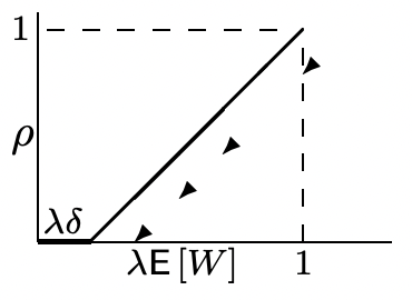
The relation between \(\rho\) and \(\lambda \mathrm{E}[W]\) is shown in Figure 5.8, and it is seen that \(\rho<1\) for \(\lambda E[W]<1\). The extreme case where \(\lambda \delta=\lambda \mathrm{E}[W]\) is the case for which each customer requires exactly one unit of service. Since at most one customer can arrive per time increment, the state always remains at \(s=\phi\), and the delay is \(\delta\), i.e., the original increment of service received when a customer arrives.

Figure 5.8: \(\rho\) as a function of \(\lambda \mathrm{E}[W]\) for given \(\lambda \delta\).

Note that \ref{5.61} is the same as the distribution of customers in the system for the M/M/1 Markov chain in (5.40), except for the anomaly in the definition of \(\rho\) here. We then have the surprising result that if round-robin queueing is used rather than FCFS, then the distribution of the number of customers in the system is approximately the same as that for an M/M/1 queue. In other words, the slow truck effect associated with the M/G/1 queue has been eliminated.

Another remarkable feature of round-robin systems is that one can also calculate the expected delay for a customer conditional on the required service of that customer. This is done in Exercise 5.16, and it is found that the expected delay is linear in the required service.

Next we look at processor sharing by going to the limit as \(\delta \rightarrow 0\). We first eliminate the assumption that the service requirement distribution is arithmetic with span \(\delta\). Assume that the server always spends an increment of time on the customer at the front of the queue, and if service is finished before the interval of length ends, the server is idle until the next sample time. The analysis of the steady-state distribution above is still valid if we define \(\overline{F}(j)=\operatorname{Pr}\{W>j \delta\}\), and \(f(j)=\overline{F}(j)-\overline{F}(j+1)\). In this case \(\delta \sum_{i=1}^{\infty} \overline{F}(i)\) lies between \(\mathrm{E}[W]-\delta\). As \(\delta \rightarrow 0\), \(\rho=\lambda \mathrm{E}[W]\), and distribution of time in the system becomes identical to that of the M/M/1 system.