6.1: Introduction

Recall that a Markov chain is a discrete-time process {\(X_n; n \geq 0\)} for which the state at each time \(n\geq 1\) is an integer-valued random variable (rv) that is statistically dependent on \(X_0, . . . X_{n-1}\) only through \(X_{n-1}\). A countable-state Markov process¹ (Markov process for short) is a generalization of a Markov chain in the sense that, along with the Markov chain {\(X_n; n\geq 1\)}, there is a randomly-varying holding interval in each state which is exponentially distributed with a parameter determined by the current state.

To be more specific, let \(X_0=i\), \(X_1=j\), \(X_2 = k\), . . . , denote a sample path of the sequence of states in the Markov chain (henceforth called the embedded Markov chain). Then the holding interval \(U_n\) between the time that state \(X_{n-1} = \ell\) is entered and \(X_n\) is entered is a nonnegative exponential rv with parameter \(\nu_{\ell}\), \(i.e.\), for all \(u \geq 0\),

\[ \text{Pr}\{ U_n\leq u | X_{n-1}=\ell \} = 1-\exp (-\nu_{\ell}u) \nonumber \]

Furthermore, \(U_n\), conditional on \(X_{n-1}\), is jointly independent of \(X_m\) for all \(m \neq n- 1\) and of \(U_m\) for all \(m \neq n\).

If we visualize starting this process at time 0 in state \(X_0 = i\), then the first transition of the embedded Markov chain enters state \(X_1 = j\) with the transition probability \(P_{ij}\) of the embedded chain. This transition occurs at time \(U_1\), where \(U_1\) is independent of \(X_1\) and exponential with rate \(\nu_i\). Next, conditional on \(X_1 = j\), the next transition enters state \(X_2 = k\) with the transition probability \(P_{jk}\). This transition occurs after an interval \(U_2\), \(i.e.\), at time \(U_1 + U_2\), where \(U_2\) is independent of \(X_2\) and exponential with rate \(\nu_j\). Subsequent transitions occur similarly, with the new state, say \(X_n = i\), determined from the old state, say \(X_{n-1} = \ell\), via \(P_{\ell i}\), and the new holding interval \(U_n\) determined via the exponential rate \(\nu_{\ell}\). Figure 6.1 illustrates the statistical dependencies between the rv’s {\(X_n; n \geq 0\)} and {\(U_n; n\geq 1\)}.

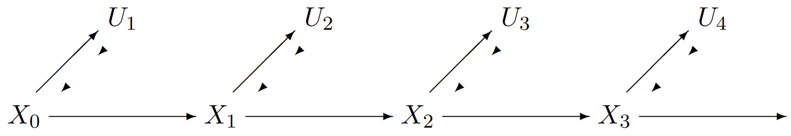
Figure 6.1: The statistical dependencies between the rv’s of a Markov process. Each holding interval \(U_i\), conditional on the current state \(X_{i-1}\), is independent of all other states and holding intervals.

The epochs at which successive transitions occur are denoted \(S_1, S_2, . . . \), so we have \(S_1 = U_1\), \(S_2 = U_1 + U_2\), and in general \(S_n = \sum^n_{m=1} U_m\) for \(n\geq 1\) wug \(S_0 = 0\). The state of a Markov process at any time \(t > 0\) is denoted by \(X(t)\) and is given by

\[ X(t) =X_n \text{ for } S_n\leq t<S_{n+1} \quad \text{for each } n\geq 0 \nonumber \]

This defines a stochastic process {\(X(t); t \geq 0\)} in the sense that each sample point \(\omega \in \Omega\) maps to a sequence of sample values of {\(X_n; n\geq 0\)} and {\(S_n; n \geq 1\)}, and thus into a sample function of {\(X(t); t\geq 0\)}. This stochastic process is what is usually referred to as a Markov process, but it is often simpler to view {\(X_n; n\geq 0\)}, {\(S_n; n\geq 1\)} as a characterization of the process. Figure 6.2 illustrates the relationship between all these quantities.

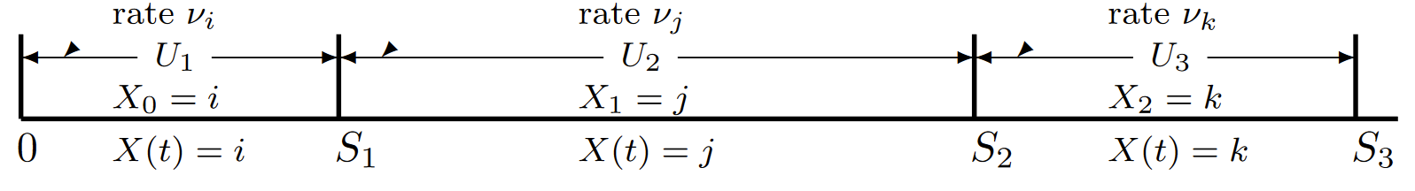
Figure 6.2: The relationship of the holding intervals {\(U_n; n\geq 1\)} and the epochs {\(S_n;n\geq 1\)} at which state changes occur. The state \(X(t)\) of the Markov process and the corresponding state of the embedded Markov chain are also illustrated. Note that if \(X_n=i\), then \(X(t)=i\) for \(S_n \leq t< S_{n+1}\)

This can be summarized in the following definition.

Definition 6.1.1. A countable-state Markov process {\(X(t); t \geq 0\)} is a stochastic process mapping each nonnegative real number \(t\) to the nonnegative integer-valued rv \(X(t)\) in such a way that for each \(t\geq 0\),

\[ X(t)=X_n \quad for \, S_n\leq t<S_{n+1} ; \quad S_0=0; \, \, S_n=\sum^n_{m=1} U_m \quad for \, \, n\geq 1 \nonumber \]

where {\(X_n; n\geq 0\)} is a Markov chain with a countably infinite or finite state space and each \(U_n\), given \(X_{n-1} = i\), is exponential with rate \(\nu_i > 0\) and is conditionally independent of all other \(U_m\) and \(X_m\).

The tacit assumptions that the state space is the set of nonnegative integers and that the process starts at \(t = 0\) are taken only for notational simplicity but will serve our needs here.

We assume throughout this chapter (except in a few places where specified otherwise) that the embedded Markov chain has no self transitions, \(i.e.\), \(P_{ii} = 0\) for all states \(i\). One reason for this is that such transitions are invisible in {\(X(t); t\geq 0\)}. Another is that with this assumption, the sample functions of {\(X(t); t\geq 0\)} and the joint sample functions of {\(X_n; n\geq 0\)} and {\(U_n; n\geq 1\)} uniquely specify each other.

We are not interested for the moment in exploring the probability distribution of \(X(t)\) for given values of \(t\), but one important feature of this distribution is that for any times \(t > \tau > 0\) and any states \(i, j\),

\[\text{Pr}\{X(t)=j|X(\tau)=i,\, \{X(s)=x(s); s<\tau\}\} = \text{Pr}\{X(t-\tau)=j|X(0)=i\} \nonumber \]

This property arises because of the memoryless property of the exponential distribution. That is, if \(X(\tau ) = i\), it makes no difference how long the process has been in state \(i\) before \(\tau\); the time to the next transition is still exponential with rate \(\nu_i\) and subsequent states and holding intervals are determined as if the process starts in state \(i\) at time 0. This will be seen more clearly in the following exposition. This property is the reason why these processes are called Markov, and is often taken as the defining property of Markov processes.

Example 6.1.1. The M/M/1 Queue: An M/M/1 queue has Poisson arrivals at a rate denoted by \(\lambda\) and has a single server with an exponential service distribution of rate \(µ >\lambda\) (see Figure 6.3). Successive service times are independent, both of each other and of arrivals. The state \(X(t)\) of the queue is the total number of customers either in the queue or in service. When \(X(t) = 0\), the time to the next transition is the time until the next arrival, \(i.e.\), \(\nu_0 = \lambda\). When \(X(t) = i\), \(i\geq 1\), the server is busy and the time to the next transition is the time until either a new arrival occurs or a departure occurs. Thus \(\nu_i = \lambda+ µ\). For the embedded Markov chain, \(P_{01} = 1\) since only arrivals are possible in state 0, and they increase the state to 1. In the other states, \(P_{i,i-1} = µ/(\lambda+µ)\) and \(P_{i,i+1} = \lambda/(\lambda+µ)\).

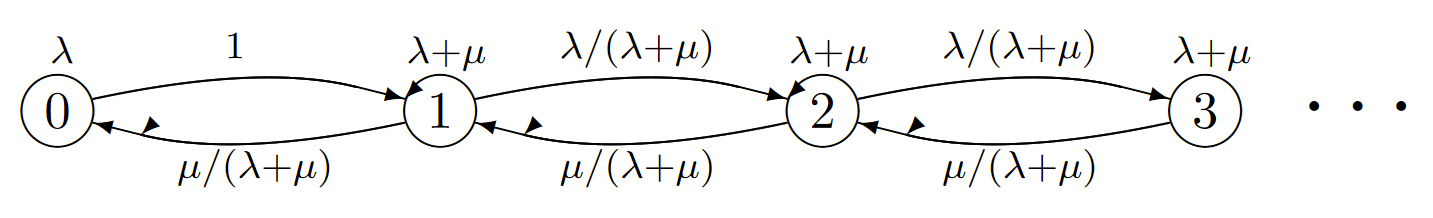
Figure 6.3: The embedded Markov chain for an M/M/1 queue. Each node \(i\) is labeled with the corresponding rate \(\nu_i\) of the exponentially distributed holding interval to the next transition. Each transition, say \(i\) to \(j\), is labeled with the corresponding transition probability \(P_{ij}\) in the embedded Markov chain.

The embedded Markov chain is a Birth-death chain, and its steady state probabilities can be calculated easily using (5.25). The result is

\[ \begin{align} &\pi_0 \, = \, \dfrac{1-\rho}{2} \qquad \text{where } \rho=\dfrac{\lambda}{\mu}\nonumber \\ &\pi_n \, = \, \dfrac{1-\rho^2}{2}\rho^{n-1} \quad \text{for } n\geq 1\end{align} \nonumber \]

Note that if \(\lambda << µ\), then \(\pi_0\) and \(\pi_1\) are each close to 1/2 (\(i.e.\), the embedded chain mostly alternates between states 0 and 1, and higher ordered states are rarely entered), whereas because of the large holding interval in state 0, the process spends most of its time in state 0 waiting for arrivals. The steady-state probability \(\pi_i\) of state \(i\) in the embedded chain is the long-term fraction of the total transitions that go to state \(i\). We will shortly learn how to find the long term fraction of time spent in state \(i\) as opposed to this fraction of transitions, but for now we return to the general study of Markov processes.

The evolution of a Markov process can be visualized in several ways. We have already looked at the first, in which for each state \(X_{n-1} = i\) in the embedded chain, the next state \(X_n\) is determined by the probabilities {\(P_{ij} ; j\geq 0\)} of the embedded Markov chain, and the holding interval \(U_n\) is independently determined by the exponential distribution with rate \(\nu_i\).

For a second viewpoint, suppose an independent Poisson process of rate \(\nu_i > 0\) is associated with each state \(i\). When the Markov process enters a given state \(i\), the next transition occurs at the next arrival epoch in the Poisson process for state \(i\). At that epoch, a new state is chosen according to the transition probabilities \(P_{ij}\). Since the choice of next state, given state \(i\), is independent of the interval in state \(i\), this view describes the same process as the first view.

For a third visualization, suppose, for each pair of states \(i\) and \(j\), that an independent Poisson process of rate \(\nu_i P_{ij}\) is associated with a possible transition to \(j\) conditional on being in \(i\). When the Markov process enters a given state \(i\), both the time of the next transition and the choice of the next state are determined by the set of \(i\) to \(j\) Poisson processes over all possible next states \(j\). The transition occurs at the epoch of the first arrival, for the given \(i\), to any of the \(i\) to \(j\) processes, and the next state is the \(j\) for which that first arrival occurred. Since such a collection of independent Poisson processes is equivalent to a single process of rate \(\nu_i\) followed by an independent selection according to the transition probabilities \(P_{ij}\), this view again describes the same process as the other views.

It is convenient in this third visualization to define the rate from any state \(i\) to any other state \(j\) as

\[q_{ij} = \nu_i P_{ij} \nonumber \]

If we sum over \(j\), we see that \(\nu_i\) and \(P_{ij}\) are also uniquely determined by {\(q_{ij} ; i, j\geq 0\)} as

\[ \nu_i = \sum_j q_{ij}; \qquad P_{ij}=q_{ij}/\nu_i \nonumber \]

This means that the fundamental characterization of the Markov process in terms of the \(P_{ij}\) and the \(\nu_i\) can be replaced by a characterization in terms of the set of transition rates \(q_{ij}\). In many cases, this is a more natural approach. For the M/M/1 queue, for example, \(q_{i,i+1}\) is simply the arrival rate \(\lambda\). Similarly, \(q_{i,i-1}\) is the departure rate \(µ\) when there are customers to be served, \(i.e.\), when \(i > 0\). Figure 6.4 shows Figure 6.3 incorporating this notational simplification.

Note that the interarrival density for the Poisson process, from any given state \(i\) to other state \(j\), is given by \(q_{ij} \exp (-q_{ij}x)\). On the other hand, given that the process is in state \(i\), the probability density for the interval until the next transition, whether conditioned on the next state or not, is \(\nu_i \exp(-\nu_ix)\) where \(\nu_i = \sum_j q_{ij}\). One might argue, incorrectly, that, conditional on the next transition being to state \(j\), the time to that transition has density \(q_{ij} \exp (-q_{ij}x)\). Exercise 6.1 uses an M/M/1 queue to provide a guided explanation of why this argument is incorrect.

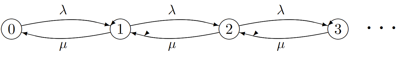
Figure 6.4: The Markov process for an M/M/1 queue. Each transition (\(i, j\)) is labelled with the corresponding transition rate \(q_{ij}\).

Sampled-Time Approximation to a Markov Process

As yet another way to visualize a Markov process, consider approximating the process by viewing it only at times separated by a given increment size \(\delta\). The Poisson processes above are then approximated by Bernoulli processes where the transition probability from \(i\) to \(j\) in the sampled-time chain is defined to be \(q_{ij}\delta\) for all \(j \neq i\).

The Markov process is then approximated by a Markov chain. Since each \(\delta q_{ij}\) decreases with decreasing \(\delta\), there is an increasing probability of no transition out of any given state in the time increment \(\delta\). These must be modeled with self-transition probabilities, say \(P_{ii}(\delta)\) which must satisfy

\[ P_{ii}(\delta) =1-\sum_jq_{ij}\delta =1-\nu_i\delta \qquad \text{for each } i\geq 0 \nonumber \]

This is illustrated in Figure 6.5 for the M/M/1 queue. Recall that this sampled-time M/M/1 Markov chain was analyzed in Section 5.4 and the steady-state probabilities were shown to be

\[ p_i(\delta) = (1-\rho)\rho^i \qquad \text{for all } i\geq 0 \quad \text{where } \rho = \lambda/\mu \nonumber \]

We have denoted the steady-state probabilities here by \(p_i(\delta)\) to avoid confusion with the steady-state probabilities for the embedded chain. As discussed later, the steady-state probabilities in \ref{6.6} do not depend on \(\delta\), so long as \(\delta \) is small enough that the self-transition probabilities are nonnegative

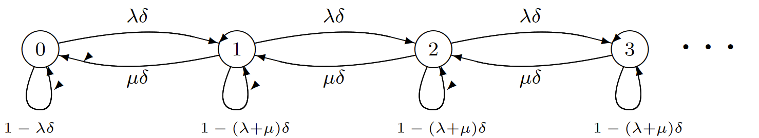
Figure 6.5: Approximating an M/M/1 queue by a sampled-time Markov chain.

This sampled-time approximation is an approximation in two ways. First, transitions occur only at integer multiples of the increment \(\delta\), and second, \(q_{ij}\delta\) is an approximation to \(\text{Pr}\{X(\delta)=j | X(0)=i\}\). From (6.3), \(\text{Pr}\{ X(\delta)=j | X(0) = i\} = q_{ij}\delta + o(\delta)\), so this second approximation is increasingly good as \(\delta \rightarrow 0\).

As observed above, the steady-state probabilities for the sampled-time approximation to an M/M/1 queue do not depend on \(\delta\). As seen later, whenever the embedded chain is positive recurrent and a sampled-time approximation exists for a Markov process, then the steadystate probability of each state \(i\) is independent of \(\delta\) and represents the limiting fraction of time spent in state \(i\) with probability 1.

Figure 6.6 illustrates the sampled-time approximation of a generic Markov process. Note that \(P_{ii}(\delta )\) is equal to \(1 -\delta \nu_i\) for each \(i\) in any such approximation, and thus it is necessary for \(\delta\) to be small enough to satisfy \(\nu_i\delta\leq 1\) for all \(i\). For a finite state space, this is satisfied for any \(\delta\leq [\max_i \nu_i]^{-1}\). For a countably infinite state space, however, the sampled-time approximation requires the existence of some finite \(B\) such that \(\nu_i\leq B\) for all \(i\). The consequences of having no such bound are explored in the next section.

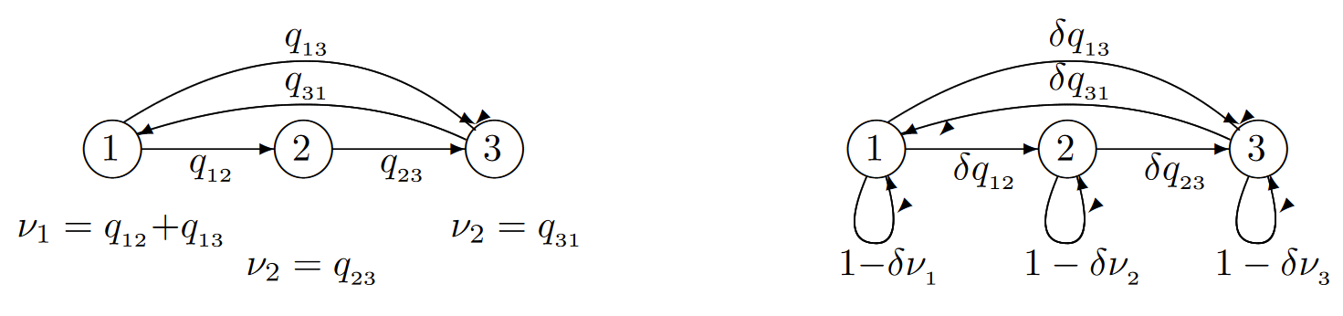
Figure 6.6: Approximating a generic Markov process by its sampled-time Markov chain.

_______________________________________________

1. These processes are often called continuous-time Markov chains.