6.2: Steady State Behavior of Irreducible Markov Processes

Definition 6.2.1 (Irreducible Markov processes) An irreducible Markov process is a Markov process for which the embedded Markov chain is irreducible (\(i.e.\), all states are in the same class).

The analysis in this chapter is restricted almost entirely to irreducible Markov processes. The reason for this restriction is not that Markov processes with multiple classes of states are unimportant, but rather that they can usually be best understood by first looking at the embedded Markov chains for the various classes making up that overall chain.

We will ask the same types of steady-state questions for Markov processes as we asked about Markov chains. In particular, under what conditions is there a set of steady-state probabilities, \(p_0, p_1, . . .\) with the property that for any given starting state \(i\), the limiting fraction of time spent in any given state \(j\) is \(p_j\) with probability 1? Do these probabilities also have the property that \(p_j = \lim_{t\rightarrow \infty} \text{Pr}\{ X(t) = j | X_0 = i\}\)?

We will find that simply having a positive-recurrent embedded Markov chain is not quite enough to ensure that such a set of probabilities exists. It is also necessary for the embedded chain steady-state probabilities {\(\pi_i; i\geq 0\)} and the holding-interval parameters {\(\nu_i;i\geq 0\)} to satisfy \(\sum_i \pi_i/\nu_i < \infty\). We will interpret this latter condition as asserting that the limiting long-term rate at which transitions occur must be strictly positive. Finally we will show that when these conditions are satisfied, the steady-state probabilities for the process are related to those of the embedded chain by

\[ p_j = \dfrac{\pi_j/\nu_j}{\sum_k\pi_k/\nu_k} \nonumber \]

Definition 6.2.2 The steady-state process probabilities, \(p_0, p_1, . . .\) for a Markov process are a set of numbers satisfying (6.2.1), where {\(\pi_i; i\geq 0\)} and {\(\nu_i; i\geq 0\)} are the steady-state probabilities for the embedded chain and the holding-interval rates respectively.

As one might guess, the appropriate approach to answering these questions comes from applying renewal theory to various renewal processes associated with the Markov process. Many of the needed results for this have already been developed in looking at the steady-state behavior of countable-state Markov chains.

We start with a very technical lemma that will perhaps appear obvious, and the reader is welcome to ignore the proof until perhaps questioning the issue later. The lemma is not restricted to irreducible processes, although we only use it in that case.

Lemma 6.2.1 Consider a Markov process for which the embedded chain starts in some given state \(i\). Then the holding time intervals, \(U_1, U_2, . . .\) are all rv’s. Let \(M_i(t)\) be the number of transitions made by the process up to and including time \(t\). Then with probability 1 (WP1),

\[ \lim_{t\rightarrow\infty} M_i(t)=\infty \nonumber \]

Proof: The first holding interval \(U_1\) is exponential with rate \(\nu_i > 0\), so it is clearly a rv (\(i.e.\), not defective). In general the state after the (\(n-1\))th transition has the PMF \(P^{n-1}_{ij}\), so the complementary distribution function of \(U_n\) is

\[\begin{aligned} \text{Pr}\{U_n>u\} \quad &= \quad \lim_{k\rightarrow \infty} \sum^k_{j=1} P^{n-1}_{ij} \exp (-\nu_ju) \\ &\leq \quad \sum^k_{j=1} P^{n-1}_{ij} \exp(-\nu_j u)+ \sum^{\infty}_{j=k+1} P^{n+1}_{ij} \quad \text{for every } k \end{aligned} \nonumber \]

For each \(k\), the first sum above approaches 0 with increasing \(u\) and the second sum approaches 0 with increasing \(k\) so the limit as \(u \rightarrow\infty\) must be 0 and \(U_n\) is a rv

It follows that each \(S_n = U_1 + · · · + U_n\) is also a rv. Now {\(S_n; n\geq 1\)} is the sequence of arrival epochs in an arrival process, so we have the set equality {\(S_n \leq t\)} = {\(M_i(t)\geq n\)} for each choice of \(n\). Since \(S_n\) is a rv, we have \(\lim_{t\rightarrow \infty} \text{Pr}\{S_n \leq t\} = 1\) for each \(n\). Thus \(\lim_{t\rightarrow \infty} \text{Pr}\{M_i(t)\geq n\} = 1\) for all \(n\). This means that the set of sample points \(\omega\) for which \(\lim_{t\rightarrow\infty} M_i(t, \omega) < n\) has probability 0 for all \(n\), and thus \(\lim_{t\rightarrow \infty} M_i(t, \omega) = \infty\) WP1.

\(\square\)

Renewals on Successive Entries to a Given State

For an irreducible Markov process with \(X_0 = i\), let \(M_{ij} (t)\) be the number of transitions into state \(j\) over the interval \((0,t]\). We want to find when this is a delayed renewal counting process. It is clear that the sequence of epochs at which state \(j\) is entered form renewal points, since they form renewal points in the embedded Markov chain and the holding intervals between transitions depend only on the current state. The questions are whether the first entry to state \(j\) must occur within some finite time, and whether recurrences to \(j\) must occur within finite time. The following lemma answers these questions for the case where the embedded chain is recurrent (either positive recurrent or null recurrent).

_______________________________________________________________________________________________

Lemma 6.2.2. Consider a Markov process with an irreducible recurrent embedded chain {\(X_n; n \geq 0\)}. Given \(X_0 = i\), let {\(M_{ij} (t); t\geq 0\)} be the number of transitions into a given state \(j\) in the interval \((0,t]\). Then {\(M_{ij} (t); t\geq 0\)} is a delayed renewal counting process (or an ordinary renewal counting process if \(j = i\)).

Proof: Given \(X_0 = i\), let \(N_{ij} (n)\) be the number of transitions into state \(j\) that occur in the embedded Markov chain by the \(n^{th}\) transition of the embedded chain. From Lemma 5.1.4, {\(N_{ij} (n); n\geq 0\)} is a delayed renewal process, so from Lemma 4.8.2, \(\lim_{n\rightarrow \infty} N_{ij} \ref{n} = \infty\) with probability 1. Note that \(M_{ij} \ref{t} = N_{ij} (M_i(t))\), where \(M_i(t)\) is the total number of state transitions (between all states) in the interval \((0,t]\). Thus, with probability 1,

\[ \lim_{t\rightarrow \infty} M_{ij}(t)=\lim_{t\rightarrow\infty} N_{ij}(M_i(t))=\lim_{n\rightarrow\infty}N_{ij}(n) = \infty \nonumber \]

where we have used Lemma 6.2.1, which asserts that \(\lim_{t\rightarrow\infty} M_i(t) = \infty\) with probability 1.

It follows that the interval \(W_1\) until the first transition to state \(j\), and the subsequent interval \(W_2\) until the next transition to state \(j\), are both finite with probability 1. Subsequent intervals have the same distribution as \(W_2\), and all intervals are independent, so {\(M_{ij} (t); t \geq 0\)} is a delayed renewal process with inter-renewal intervals {\(W_k; k\geq 1\)}. If \(i = j\), then all \(W_k\) are identically distributed and we have an ordinary renewal process, completing the proof.

\(\square \)

The inter-renewal intervals \(W_2, W_3, . . .\) for {\(M_{ij} (t); t\geq 0\)} above are well-defined nonnegative IID rv’s whose distribution depends on \(j\) but not \(i\). They either have an expectation as a finite number or have an infinite expectation. In either case, this expectation is denoted as \(\mathsf{E} [W(j)] = \overline{W}(j)\). This is the mean time between successive entries to state \(j\), and we will see later that in some cases this mean time can be infinite.

Limiting Fraction of Time in Each State

In order to study the fraction of time spent in state \(j\), we define a delayed renewal-reward process, based on {\(M_{ij} (t); t \geq 0\)}, for which unit reward is accumulated whenever the process is in state \(j\). That is (given \(X_0 = i\)), \(R_{ij} \ref{t} = 1\) when \(X(t) = j\) and \(R_{ij} \ref{t} = 0\) otherwise. (see Figure 6.7). Given that transition \(n-1\) of the embedded chain enters state \(j\), the interval \(U_n\) is exponential with rate \(\nu_j\), so \(\mathsf{E} [U_n | X_{n-1}=j] = 1/\nu_j\).

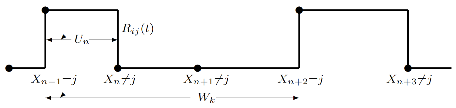
Figure 6.7: The delayed renewal-reward process {\(R_{ij} (t); t \geq 0\)} for any time in state \(j\). The reward is one whenever the process is in state \(j\), \(i.e.\), \(R_{ij}(t)=\mathbb{I}_{\{X(t)=j\}}\). A renewal occurs on each entry to state \(j\), so the reward starts at each such entry and continues until a state transition, assumed to enter a state other than \(j\). The reward then ceases until the next renewal, \(i.e.\), the next entry to state \(j\). The figure illustrates the \(k\)th inter-renewal interval, of duration \(W_k\), which is assumed to start on the \(n-1\)st state transition. The expected interval over which a reward is accumulated is \(\nu_j\) and is the expected duration of the inter-renewal interval is \(\overline{W}(j)\).

Let \(p_j (i)\) be the limiting time-average fraction of time spent in state \(j\). We will see later that such a limit exists WP1, that the limit does not depend on \(i\), and that it is equal to the steady-state probability \(p_j\) in (6.2.1). Since \(\overline{U}(j) = 1/\nu_j\), Theorems 4.4.1 and 4.8.4, for ordinary and delayed renewal-reward processes respectively, state that¹

\[ \begin{align} p_j(i) \quad &= \quad \lim_{t\rightarrow \infty} \dfrac{\int^t_0 R_{ij}(\tau)d\tau}{t} \quad \text{WP1} \\ &= \quad \dfrac{\overline{U}(j)}{\overline{W}(j)} \quad = \quad \dfrac{1}{\nu_j\overline{W}(j)} \end{align} \nonumber \]

This shows that the limiting time average, \(p_j (i)\), exists with probability 1 and is independent of the starting state \(i\). We show later that it is the steady-state process probability given by (6.2.1). We can also investigate the limit, as \(t \rightarrow \infty\), of the probability that \(X(t) = j\). This is equal to \(\lim_{t\rightarrow \infty} \mathsf{E} [R(t)]\) for the renewal-reward process above. Because of the exponential holding intervals, the inter-renewal times are non-arithmetic, and from Blackwell’s theorem, in the form of (4.105),

\[ \lim_{t\rightarrow\infty} \text{Pr}\{X(t)=j \} = \dfrac{1}{\nu_j\overline{W}(j)} = p_j(i) \nonumber \]

We summarize these results in the following lemma.

Lemma 6.2.3 Consider an irreducible Markov process with a recurrent embedded Markov chain starting in \(X_0 = i\). Then with probability 1, the limiting time average in state \(j\) is given by \(p_j \ref{i} = \dfrac{1}{\nu_j\overline{W}(j)}\). This is also the limit, as \(t \rightarrow \infty\), of \(\text{Pr}\{ X(t) = j\}\).

Finding \(\{p_j (i); j\geq 0\}\) in terms of \(\{\pi_j ; j\geq 0\}\)

Next we must express the mean inter-renewal time, \(\overline{W}(j)\), in terms of more accessible quantities that allow us to show that \(p_j \ref{i} = p_j\) where \(p_j\) is the steady-state process probability of Definition 6.2.2. We now assume that the embedded chain is not only recurrent but also positive recurrent with steady-state probabilities {\(\pi_j ; j\geq 0\)}. We continue to assume a given starting state \(X_0 = i\). Applying the strong law for delayed renewal processes (Theorem 4.8.1) to the Markov process,

\[ \lim_{t\rightarrow\infty} M_{ij}(t)/t=1/\overline{W}(j) \qquad \text{WP1} \nonumber \]

As before, \(M_{ij} \ref{t} = N_{ij} (M_i(t))\). Since \(\lim_{t\rightarrow\infty} M_i(t) = \infty\) with probability 1,

\[ \lim_{t\rightarrow\infty}\dfrac{M_{ij}(t)}{M_i(t)} = \lim_{t\rightarrow\infty}\dfrac{N_{ij}(M_i(t))}{M_i(t)} = \lim_{n\rightarrow\infty} \dfrac{N_{ij}(n)}{n}=\pi_j \qquad \text{WP1} \nonumber \]

In the last step, we applied the same strong law to the embedded chain. Combining (6.2.6) and (6.2.7), the following equalities hold with probability 1.

\[ \begin{align} \dfrac{1}{\overline{W}(j)} \quad &= \quad \lim_{t\rightarrow\infty}\dfrac{M_{ij}(t)}{t} \nonumber \\ &= \quad \lim_{t\rightarrow\infty} \dfrac{M_{ij}(t)}{M_i(t)}\dfrac{M_i(t)}{t} \nonumber \\ &= \quad \pi_j \lim_{t\rightarrow \infty} \dfrac{M_i(t)}{t} \end{align} \nonumber \]

This tells us that \(\overline{W}(j)\pi_j\) is the same for all \(j\). Also, since \(\pi_j > 0\) for a positive recurrent chain, it tell us that if \(\overline{W}(j) < \infty\) for one state \(j\), it is finite for all states. Also these expected recurrence times are finite if and only if \(\lim_{t\rightarrow\infty} M_i(t)/t > 0\). Finally, it says implicitly that \(\lim_{t\rightarrow\infty}M_i(t)/t\) exists WP1 and has the same value for all starting states \(i\).

There is relatively little left to do, and the following theorem does most of it.

Theorem 6.2.1. Consider an irreducible Markov process with a positive recurrent embedded Markov chain. Let {\(\pi_j ; j\geq 0\)} be the steady-state probabilities of the embedded chain and let \(X_0 = i\) be the starting state. Then, with probability 1, the limiting time-average fraction of time spent in any arbitrary state \(j\) is the steady-state process probability in (6.2.1), \(i.e.\),

\[ p_j(i)=p_j=\dfrac{\pi_k/\nu_j}{\sum_k\pi_k/\nu_k} \nonumber \]

The expected time between returns to state \(j\) is

\[ \overline{W}(j) = \dfrac{\sum_k \pi_k/\nu_k}{\pi_j} \nonumber \]

and the limiting rate at which transitions take place is independent of the starting state and given by

\[ \lim_{t\rightarrow\infty} \dfrac{M_i(t)}{t} = \dfrac{1}{\sum_k\pi_k/\nu_k} \qquad \text{WP1} \nonumber \]

Discussion: Recall that \(p_j (i)\) was defined as a time average WP1, and we saw earlier that this time average existed with a value independent of \(i\). The theorem states that this time average (and the limiting ensemble average) is given by the steady-state process probabilities in (6.2.1). Thus, after the proof, we can stop distinguishing these quantities.

At a superficial level, the theorem is almost obvious from what we have done. In particular, substituting (6.2.8) into (6.2.3), we see that

\[ p_j(i) = \dfrac{\pi_j}{\nu_j} \lim_{t\rightarrow\infty} \dfrac{M_i(t)}{t} \qquad \text{WP1} \nonumber \]

Since \(p_j \ref{i} = \lim_{t\rightarrow\infty} \text{Pr}\{ X(t) = j\}\), and since \(X(t)\) is in some state at all times, we would conjecture (and even insist if we didn’t read on) that \(\sum_j p_j \ref{i} = 1\). Adding that condition to normalize (6.2.10), we get (6.2.9), and (6.2.10) and (6.2.11) follow immediately. The trouble is that if \(\sum_j \pi_j/\nu_j = \infty\), then (6.2.9) says that \(p_j = 0\) for all \(j\), and (6.2.11) says that \(\lim M_i(t)/t = 0\), \(i.e.\), the process ‘gets tired’ with increasing \(t\) and the rate of transitions decreases toward 0. The rather technical proof to follow deals with these limits more carefully

Proof: We have seen in (6.2.8) that \(\lim_{t\rightarrow\infty} M_i(t)/t\) is equal to a constant, say \(\alpha\), with probability 1 and that this constant is the same for all starting states \(i\). We first consider the case where \(\alpha > 0\). In this case, from (6.2.8), \(\overline{W}(j) < \infty\) for all \(j\). Choosing any given \(j\) and any positive integer \(\ell\), consider a renewal-reward process with renewals on transitions to \(j\) and a reward \(R^{\ell}_{ij} \ref{t} = 1\) when \(X(t) \leq \ell\). This reward is independent of \(j\) and equal to \(\sum^{\ell}_{k=1} R_{ik}(t)\). Thus, from (6.2.3), we have

\[ \lim_{t\rightarrow\infty} \dfrac{\int^t_0 R^{\ell}_{ij} (\tau) d\tau}{t} = \sum^{\ell}_{k=1} p_k(i) \nonumber \]

If we let \(\mathsf{E} \left[ R^{\ell}_j\right] \) be the expected reward over a renewal interval, then, from Theorem 4.8.4,

\[\lim_{t\rightarrow\infty}\dfrac{\int^t_0 R^{\ell}_{ij}(\tau)d\tau}{t} = \dfrac{\mathsf{E}\left[ R^{\ell}_j \right] }{\overline{U}_j} \nonumber \]

Note that \(\mathsf{E} \left[ R^{\ell}_j\right]\) above is non-decreasing in \(\ell\) and goes to the limit \(\overline{W}(j)\) as \(\ell \rightarrow \infty\). Thus, combining (6.2.11) and (6.2.14), we see that

\[ \lim_{\ell \rightarrow\infty} \sum^{\ell}_{k=1} p_k(i) =1 \nonumber \]

With this added relation, (6.2.9), (6.2.10), and (6.2.11) follow as in the discussion. This completes the proof for the case where \(\alpha > 0\).

For the remaining case, where \(\lim_{t\rightarrow\infty} M_i(t)/t = \alpha = 0\), (6.2.8) shows that \(\overline{W}(j) = \infty\) for all \(j\) and (6.2.12) then shows that \(p_j \ref{i} = 0\) for all \(j\). We give a guided proof in Exercise 6.6 that, for \(\alpha = 0\), we must have \(\sum_i \pi_i/\nu_i = \infty\). It follows that (6.2.9), (6.2.10), and (6.2.11) are all satisfied.

\(\square\)

This has been quite a difficult proof for something that might seem almost obvious for simple examples. However, the fact that these time-averages are valid over all sample points with probability 1 is not obvious and the fact that \(\pi_j\overline{W}(j)\) is independent of \(j\) is certainly not obvious.

The most subtle thing here, however, is that if \(\sum_i \pi_i/\nu_i = \infty\), then \(p_j = 0\) for all states \(j\). This is strange because the time-average state probabilities do not add to 1, and also strange because the embedded Markov chain continues to make transitions, and these transitions, in steady state for the Markov chain, occur with the probabilities \(\pi_i\). Example 6.2.1 and Exercise 6.3 give some insight into this. Some added insight can be gained by looking at the embedded Markov chain starting in steady state, \(i.e.\), with probabilities {\(\pi_i; i\geq 0\)}. Given \(X_0 = i\), the expected time to a transition is \(1/\nu_i\), so the unconditional expected time to a transition is \(\sum_i \pi_i/\nu_i\), which is infinite for the case under consideration. This is not a phenomenon that can be easily understood intuitively, but Example 6.2.1 and Exercise 6.3 will help.

Solving for the steady-state process probabilities directly

Let us return to the case where \(\sum_k \pi_k/\nu_k < \infty\), which is the case of virtually all applications. We have seen that a Markov process can be specified in terms of the time-transitions \(q_{ij} = \nu_iP_{ij}\), and it is useful to express the steady-state equations for \(p_j\) directly in terms of \(q_{ij}\) rather than indirectly in terms of the embedded chain. As a useful prelude to this, we first express the \(\pi_j\) in terms of the \(p_j\). Denote \(\sum_k \pi_k/\nu_k\) as \(\beta< \infty\). Then, from (6.2.9), \(p_j = \pi_j/\nu_j\), so \(\pi_j = p_j\nu_j \beta\). Expressing this along with the normalization \(\sum_k \pi_k = 1\), we obtain

\[ \pi_i = \dfrac{p_i\nu_i}{\sum_k p_k\nu_k} \nonumber \]

Thus, \(\beta= 1/ \sum_k p_k\nu_k\), so

\[\sum_k \pi_k/\nu_k = \dfrac{1}{\sum_k p_k \nu_k} \nonumber \]

We can now substitute \(\pi_i\) as given by (6.2.15) into the steady-state equations for the embedded Markov chain, \(i.e.\), \(\pi_j = \sum_i \pi_iP_{ij}\) for all \(j\), obtaining

\[ p_j\nu_j = \sum_i p_i\nu_i P_{ij} \nonumber \]

for each state \(j\). Since \(\nu_iP_{ij} = q_{ij} \),

\[ p_j\nu_j = \sum_i p_iq_{ij}; \qquad \sum_ip_i=1 \nonumber \]

This set of equations is known as the steady-state equations for the Markov process. The normalization condition \(\sum_i p_i = 1\) is a consequence of (6.2.16) and also of (6.2.9). Equation (6.2.17) has a nice interpretation in that the term on the left is the steady-state rate at which transitions occur out of state \(j\) and the term on the right is the rate at which transitions occur into state \(j\). Since the total number of entries to \(j\) must differ by at most 1 from the exits from \(j\) for each sample path, this equation is not surprising.

The embedded chain is positive recurrent, so its steady-state equations have a unique solution with all \(\pi_i > 0\). Thus (6.2.17) also has a unique solution with all \(p_i > 0\) under the the added condition that \(\sum_i \pi_i/\nu_i < \infty\). However, we would like to solve (6.2.17) directly without worrying about the embedded chain

If we find a solution to (6.2.17), however, and if \(\sum_i p_i\nu_i < \infty\) in that solution, then the corresponding set of \(\pi_i\) from (6.2.15) must be the unique steady-state solution for the embedded chain. Thus the solution for \(p_i\) must be the corresponding steady-state solution for the Markov process. This is summarized in the following theorem.

Theorem 6.2.2. Assume an irreducible Markov process and let {\(p_i; i\geq 0\)} be a solution to (6.2.17). If \(\sum_i p_i\nu_i < \infty\), then, first, that solution is unique, second, each \(p_i\) is positive, and third, the embedded Markov chain is positive recurrent with steady-state probabilities satisfying (6.2.15). Also, if the embedded chain is positive recurrent, and \(\sum_i \pi_i/\nu_i < \infty\) then the set of \(p_i\) satisfying (6.2.9) is the unique solution to (6.2.17).

sampled-time approximation again

For an alternative view of the probabilities {\(p_i; i\geq 0\)}, consider the special case (but the typical case) where the transition rates {\(\nu_i; i\geq 0\)} are bounded. Consider the sampled-time approximation to the process for a given increment size \(\delta \leq [\max_i \nu_i]^{-1}\) (see Figure 6.6). Let {\(p_i(\delta); i\geq 0\)} be the set of steady-state probabilities for the sampled-time chain, assuming that they exist. These steady-state probabilities satisfy

\[ p_j(\delta) = \sum_{i\neq j} p_i(\delta)q_{ij}\delta+p_j(\delta)(1-\nu_j\delta); \quad p_j(\delta) \geq 0; \quad \sum_j p_j(\delta) =1 \nonumber \]

The first equation simplifies to \(p_j (\delta)\nu_j = \sum_{i\neq j} p_i(\delta)q_{ij} \), which is the same as (6.2.17). It follows that the steady-state probabilities {\(p_i; i\geq 0\)} for the process are the same as the steady-state probabilities {\(p_i(\delta); i\geq 0\)} for the sampled-time approximation. Note that this is not an approximation; \(p_i(\delta)\) is exactly equal to \(p_i\) for all values of \(\delta \leq 1/ \sup_i \nu_i\). We shall see later that the dynamics of a Markov process are not quite so well modeled by the sampled time approximation except in the limit \(\delta\rightarrow 0\).

Pathological cases

Example 6.2.1 (Zero Transition Rate) Consider the Markov process with a positive-recurrent embedded chain in Figure 6.8. This models a variation of an M/M/1 queue in which the server becomes increasingly rattled and slow as the queue builds up, and the customers become almost equally discouraged about entering. The downward drift in the transitions is more than overcome by the slow-down in large numbered states. Transitions continue to occur, but the number of transitions per unit time goes to 0 with increasing time. Although the embedded chain has a steady-state solution, the process can not be viewed as having any sort of steady state. Exercise 6.3 gives some added insight into this type of situation.

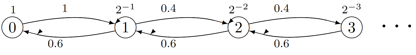
Figure 6.8: The Markov process for a variation on M/M/1 where arrivals and services get slower with increasing state. Each node \(i\) has a rate \(\nu_i=2^{-i}\). The embedded chain transitions probabilities are \(P_{i,i+1}=0.4\) for \(i\geq 1\) and \(P_{i,i-1}=0.6\) for \(i\geq 1\), thus ensuring that the embedded Markov chain is positive recurrent. Note that \(q_{i,i+1}> q_{i+1,i}\), thus ensuring that the Markov process drifts to the right.

It is also possible for (6.2.17) to have a solution for {\(p_i; i\geq 0\)} with \(\sum_i p_i = 1\), but \(\sum_i p_i\nu_i = \infty\). This is not possible for a positive recurrent embedded chain, but is possible both if the embedded Markov chain is transient and if it is null recurrent. A transient chain means that there is a positive probability that the embedded chain will never return to a state after leaving it, and thus there can be no sensible kind of steady-state behavior for the process. These processes are characterized by arbitrarily large transition rates from the various states, and these allow the process to transit through an infinite number of states in a finite time.

Processes for which there is a non-zero probability of passing through an infinite number of states in a finite time are called irregular. Exercises 6.8 and 6.7 give some insight into irregular processes. Exercise 6.9 gives an example of a process that is not irregular, but for which (6.2.17) has a solution with \(\sum_i p_i = 1\) and the embedded Markov chain is null recurrent. We restrict our attention in what follows to irreducible Markov chains for which (6.2.17) has a solution, \(\sum p_i = 1\), and \(\sum p_i\nu_i < \infty\). This is slightly more restrictive than necessary, but processes for which \(\sum_i p_i\nu_i = \infty\) (see Exercise 6.9) are not very robust.

_________________________________________________

1. Theorems 4.4.1 and 4.8.4 do not cover the case where \(\overline{W} \ref{j} = \infty\), but, since the expected reward per renewal interval is finite, it is not hard to verify (6.2.3) in that special case.